Supplementary Information
Funding
COG-UK is supported by funding from the Medical Research Council (MRC) part of UK Research & Innovation (UKRI), the National Institute of Health Research (NIHR) and Genome Research Limited, operating as the Wellcome Sanger Institute. The Imperial College COVID-19 Research Fund, UKRI (MR/V038109/1), The Academy of Medical Sciences (SBF004/1080), Bill & Melinda Gates Foundation (OPP1197730, OPP1175094), the European Commission (CoroNAb 101003653), the NIHR BRC Imperial College NHS Trust Infection and COVID themes (RDA02), Amazon AWS and Microsoft AI for Health, the EPSRC, The Medical Research Council (MR/R015600/1), the NIHR Health Protection Research Unit for Modelling and Health Economics, NIHR VEEPED project funding (PR-OD-1017-20002). Wellcome core funding to the Wellcome Sanger Institute (206194). JTM, NL and AR acknowledge the support of the Wellcome Trust (Collaborators Award 206298/Z/17/Z – ARTIC network). AR is supported by the European Research Council (grant agreement no. 725422 – ReservoirDOCS).
Methods
Logistic growth model applied to variant frequency data
The logistic growth model fitted to VOC frequency data arises from a simple mechanistic model for competition between two strains. Let established lineages have a reproduction number R and let the VOC have reproduction number R(1+s). According to this model, the log odds of observing a variant over time will be proportional to (R/g)st, where R is assumed to be constant over weeks 44-49, g is the generation time, s is a selection coefficient (assumed to be constant) and t is time. If these conditions are met, s can be interpreted as a multiplicative change in the reproduction number or as a change in the generation time or as some combination of these factors. From available data on times of sampling each variant, the compound parameter (R/g)s can be estimated. An approximate estimate of s is obtained by treating R=1 and generation time g=6.5 days as a constant for weeks 44-49. In the text, we refer to s as the change in growth per generation, and is comparable to multiplicative changes in Rt estimated using other methods.
Phylodynamic analysis
Analysis was based on Pillar 2 whole genome sequences with known Upper Tier Local Authority (UTLA). Maximum likelihood non-parametric phylodynamic analysis was carried out by: 1) estimating a maximum likelihood phylogeny in IQtree18 (HKY model of sequence evolution); 2) We removed duplicated identical sequences and estimated a time-scaled phylogeny using treedater19 using a strict molecular clock. The molecular clock rate of evolution was constrained to 0.0005 - 0.0015 substitutions per site per year. Small branch lengths in the tree were collapsed and polytomies randomly resolved to produce 20 new variations on the dated ML tree. 3) The skygrowth model was then fitted to these dated trees with parameters 64 time steps and tau bounded between 0.0025-20. Growth rate estimates were translated to reproduction numbers using the method of Wallinga and Lipsitch20 in the epitrix R package and using serial intervals from Flaxman et al.9 The main text reports the median growth rate over time. A sensitivity analysis was carried out with the molecular clock rate fixed at 0.001 substitutions per site per year which yielded only marginally different estimates of the median growth rate.
Sequence sample weights were used to select samples for phylodynamic modelling. Weights, assigned to sequence samples according to their UTLA and their collection date, correspond to the number of confirmed cases represented by each sequence in a UTLA relative to other UTLAs on the same date. To smooth over sparsity, case and sample counts were summed over the fourteen days prior to the date. Confirmed cases were accessed from the ONS API (https://api.coronavirus.data.gov.uk). Code to compute sequence sample weights is available at GitHub - robj411/sequencing_coverage.
Bayesian coalescent phylodynamic analysis was performed using BEAST v1.10.4 (Suchard et al. 2018) employing the Skygrid non-parametric approach (Gill et al. 2013) and exponential and logistic growth parametric models. A Jukes-Cantor model of substitution and a strict molecular clock were assumed. MCMC chains were run for 100M states, removing 10M as ‘burn-in’ and then thinning to 9000 samples from the posterior. Parameters were summarised and demographic curves reconstructed using Tracer v1.7.2 (Rambaut et al. 2018).
SGTF as a biomarker for the VOC and frequency of SGTF over time
Data on SGTF among pillar 2 tests was obtained from the 3 largest (“Lighthouse”) PCR testing laboratories and integrated into the PHE Second Generation Surveillance System (SGSS) database. We also obtained the total number of cases reported by Public Health England. Application of SGTF as a diagnostic for the VOC provides a large advantage over genomic sequencing in terms of cost, speed, and the sample size of available test results. We extracted 275,571 S target positive (S+) and 96,070 S target negative (S-) test results collected between 1 October and 19 December, 2020 and examined the potential to use SGTF cases (S-) as a biomarker for the VOC lineage. While the tests are not a representative sample of infections over this time period, they are a representative sample of tests within a given region and week and thus provide information about the relative abundance of the VOC versus other variants over time and between regions.
Other lineages have been observed to carry Δ69-70 which is associated with SGTF and which would have a similar impact on the TaqPath assay. The diagnostic specificity of SGTF will therefore vary over time and space as it depends on the abundance of other lineages with Δ69-70. This deletion is mostly found in global lineage B.1.258 and is highly linked with the spike N439K variant21. Lineage B.1.258 has circulated in the UK since June 2020 where it is now widespread. However, the frequency of this variant has been relatively stable since October 2020.
In order to capture diagnostic uncertainty with SGTF, we fitted a spatio-temporal model of the frequency of the VOC relative to other variants carrying Δ69-70. We fitted a generalized additive model22,23 to counts of genomes classified 24 as belonging to the VOC lineage or genomes which do not belong to the VOC lineage but still carry Δ69-70. Counts were tabulated by LTLA and epi week. We used a cubic spline to model trends over time, and correlation between neighbouring LTLAs was modeled with a Gaussian Markov Random Field (GMRF). This model was used to predict the true positive rate (TPR) - the probability that a sample collected at a particular time and place belongs to the VOC lineage, given that it carries Δ69-70. Figure S1 shows how this prediction has changed over weeks spanning November 2020. From week 50 onwards, we assumed the TPR was 1 across England. The fitted model thus provided an estimate of the true positive rate (TPR) of using SGTF as a proxy for VOC frequency as a function of time and region in England (Figure S2).
Regression analysis of VOC transmissibility
Using reported COVID-19 PCR-positive case counts and deaths, we estimated the time-varying reproduction numbers Rt for epidemiological weeks 44-50 in each LTLA and STP in England. These estimates were obtained from a previously developed11 Bayesian semi-mechanistic transmission model with a latent weekly random walk process that does not include underlying factors that drive transmission. The STP model is based on pillar 2 cases only, and includes hospital admissions as an additional input; the LTLA model is based on both pillar 1 and pillar 2 data. Further model information can be found in previous publications9,25. These Rt estimates refer to the reproduction number of the infections that gave rise to the infections at time t. Given this definition and the approximately 1 week generation time of SARS-CoV-2, we would expect Rt to be most closely associated with VOC frequency 1 week earlier. We therefore present regressions of Rt against frequency at week t-1 for our default analysis (where t spans weeks 44-50), but present results for regression of Rt against frequency at week t as a sensitivity analysis in Supplementary Information.
We consider two data sources when estimating the proportion of the VOC: Genomic-based frequency estimates and TPR-adjusted SGTF proportions of pillar 2 cases for which S-gene data was available. For the SGTF-based estimates, frequency estimates were available for all STPs and LTLAs for the weeks 43-49 (294 STP-weeks in total). When using genomic data, 7 STP-weeks in the week range 43-49 had no sampled genomes, leaving 287 STP-weeks for analysis, for which we had an average of 137 genomes per STP week (of which on average 7 were the VOC).
We use two types of frequentist models. The first uses a fixed effect for each area, the second uses a random effect for each area. Fixed effects of epidemiological week were included in both cases. Confidence intervals for the fixed and random effects models were computed through a bootstrapping method which resamples the areas with replacement and also samples the counts of VOC in each week/area pair based on the observed counts. This bootstrap aims to account for potential skewness and non-normality of responses, dependence within areas and the randomness in the proportion of the VOC sampled within an area. When using genomic-based frequency estimates we excluded STP-weeks that had fewer than 5 genetic profiles, as these were deemed to not give reliable estimates of the proportion of VOC. This removed a further 14 out of the 287 STP-weeks from those analyses.
We also implemented a Bayesian regression model 26 at STP level, taking into account uncertainty in the frequency estimates and uncertainty in the Rt estimates. VOC frequency was modelled explicitly, such that it simultaneously informed the parameter for binomially-distributed observations of frequency and the Rt estimates. The regression for Rt included terms for the VOC frequency, the week (modelled with a smooth spline) and the area as a factor. The formula to describe the binomial frequency data includes a linear function of time with an area-dependent slope, and was fitted to the genome counts and the counts of S-negative cases separately.
| MLE %Growth difference per generation (95% confidence interval) | SGTF MLE %Growth difference per generation | |
|---|---|---|
| South East | 49 (43-55) | 54 |
| London | 49 (43-54) | 60 |
| East of England | 53 (44-62) | 67 |
| West Midlands | 59 | |
| East Midlands | 56 | |
| North West | 58 | |
| Yorkshire and The Humber | 40 | |
| North East | 75 | |
| South West | 48 |
Table S1 | Estimated growth difference per generation of B.1.1.7 by English administrative region based on a maximum likelihood estimation of logistic growth in variant frequency and assuming a 6.5 day generation time and Rt=1 for established lineages. Confidence intervals are based on likelihood profiles
| Model | Spatial Resolution | Data for Variants | Estimated effect [95% CI] |
|---|---|---|---|
| Fixed | STP | Genomic | 0.34 [0.16, 0.60] |
| Random | STP | Genomic | 0.52 [0.35, 0.85] |
| Bayes | STP | Genomic | 0.54 [0.33, 0.77] |
| Fixed | LTLA | TPR-adjusted SGTF | 0.45 [0.40, 0.59] |
| Random | LTLA | TPR-adjusted SGTF | 0.53 [0.49, 0.67] |
| Fixed | STP | TPR-adjusted SGTF | 0.35 [0.15, 0.56] |
| Random | STP | TPR-adjusted SGTF | 0.44 [0.27, 0.65] |
| Bayes | STP | TPR-adjusted SGTF | 0.43 [0.30, 0.56] |
Table S2 | Estimated additive change of reproduction numbers of VOC compared with non-VOC using different regression models, spatial resolutions, and data to estimate the prevalence of the VOC. Analyses use data on the proportion of the VOC and estimates of Rt in weeks 44-50.
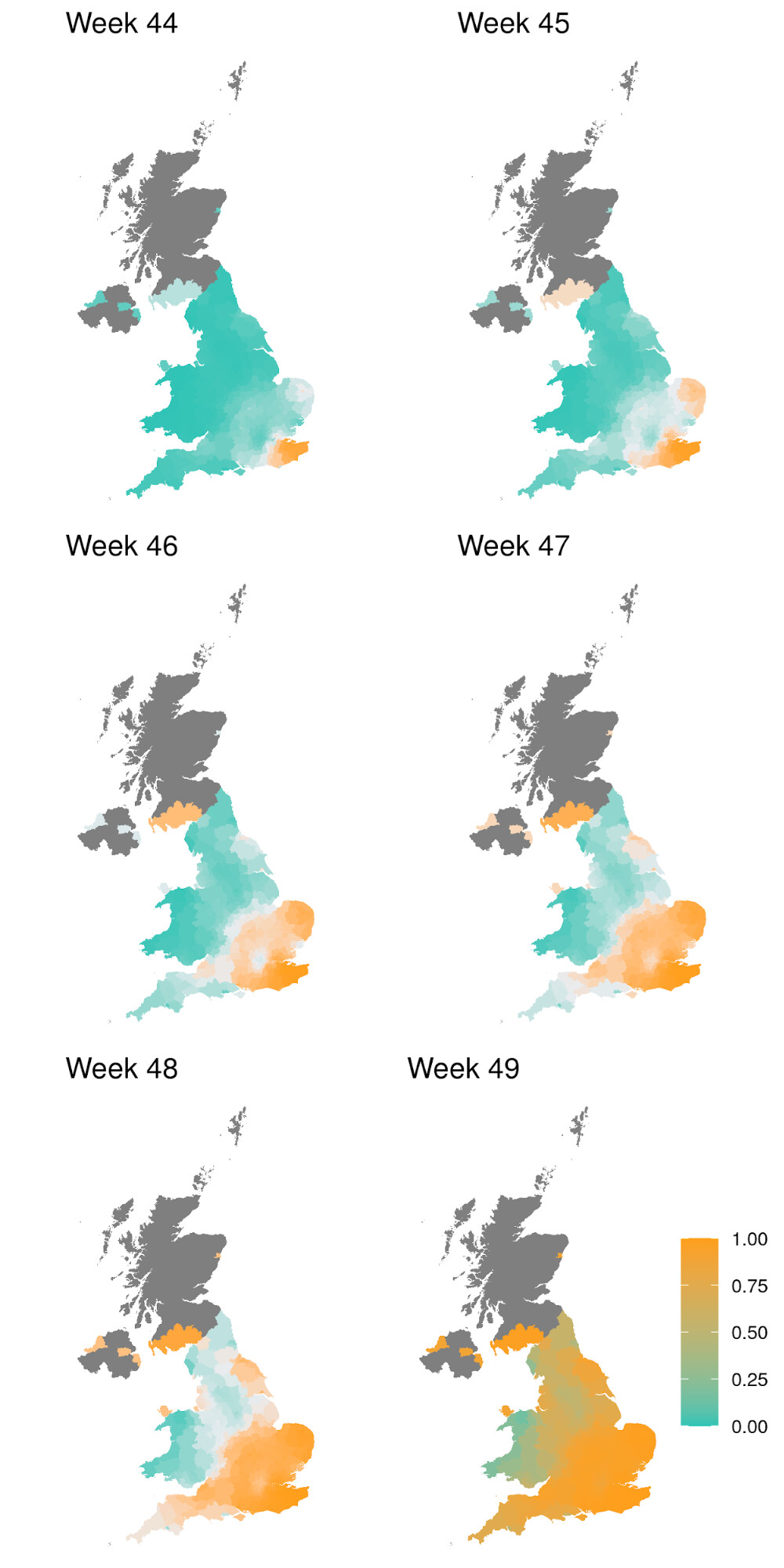
Figure S1 | Estimate of true positive rates for classification of B.1.1.7 infection given SGTF result (S-) as a function of time and UK region. The colour gradient shows the probability of sampling a B.1.1.7 sequence conditional on sampling any sequence with Δ69-70.
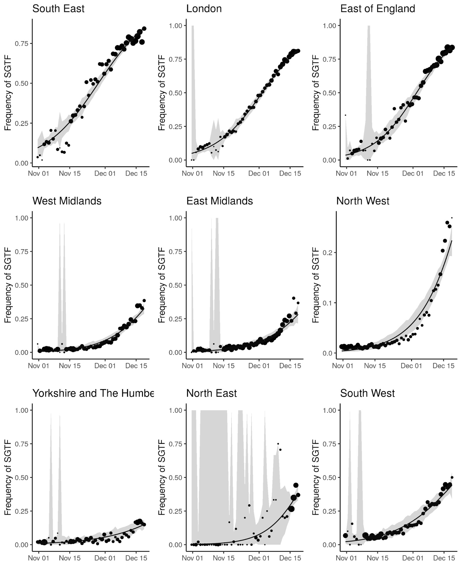
Figure S2 | Empirical (point) and estimated (line) frequencies of TPR-adjusted SGTF frequencies over time. The size of points correspond to the number of samples observed by day. Confidence intervals show 95% estimated sampling error for daily proportions.

Figure S3 | Case trends in all NHS STP areas, ordered by decreasing frequency of S- in the last week shown. Total cases reported are shown as a thick line. A subset of these - those tested in the 3 largest “Lighthouse” laboratories - were tested for SGTF. The total cases line is coloured according to percentage S- among those tested. Counts of S+ and S- reported via the PHE SGSS system are shown by the thin lines. The dates of the second lockdown are indicated by the vertical red lines. Raw SGTF data are shown here (not adjusted for TPR), so S- cases in earlier weeks include other non-VOC lineages, especially outside the East and South East of England.
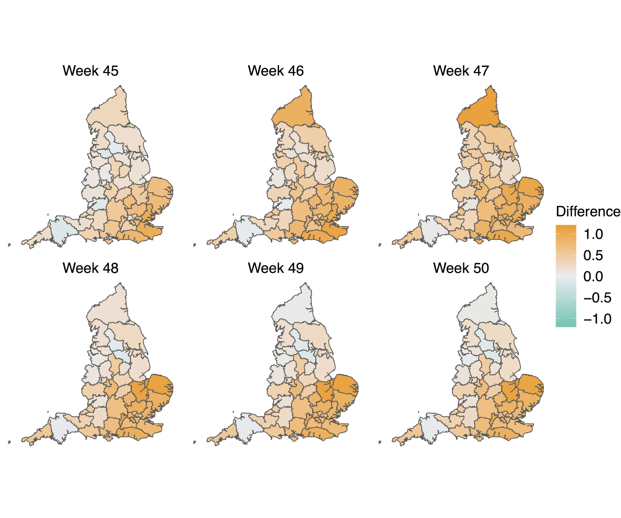
Figure S4 | Map of the difference in median Rt estimates for VOC and non-VOC variants for all STPs between week 45 to week 50. The darker orange color indicates the additive advantage VOC has over non-VOC variant for Rt, whereas the darker green color shows the advantage for non-VOC variant over VOC.

Figure S5 | Map of the ratio of median Rt estimates for VOC and non-VOC variants for all STPs between week 45 to week 50. Darker color indicates the higher multiplicative advantage for VOC variant in comparison to the non-VOC variant. The mean of the ratio between R estimates for S- and S+ for all posterior samples across weeks 45 to 50 and all STPs is 1.56, with 95% CI [0.92 - 2.28].
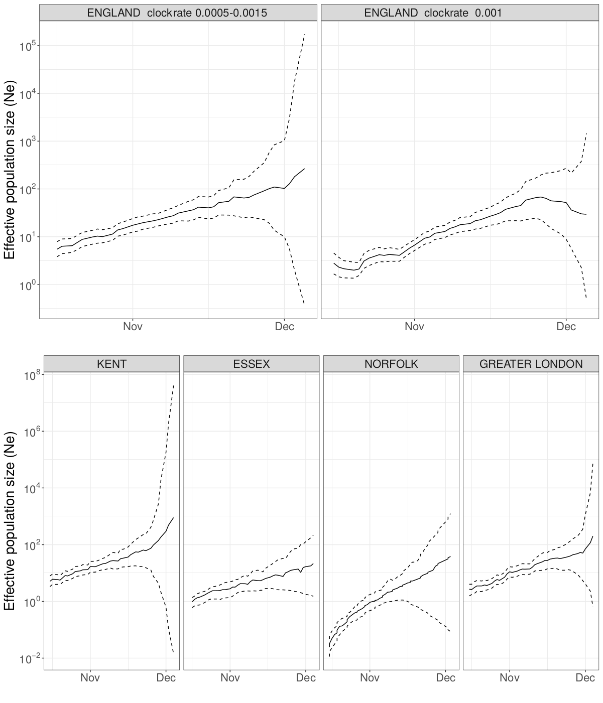
Figure S6 | Maximum likelihood skygrowth estimates of the effective population size of the VOC through time in England and in four areas of England with more than 80 whole genome sequences. In the upper right panel the molecular clock rate of evolution was fixed at 0.001 substitutions per site per year. In all other analyses the rate was estimated and bound between 0.0005 and 0.0015 substitutions per site per year.
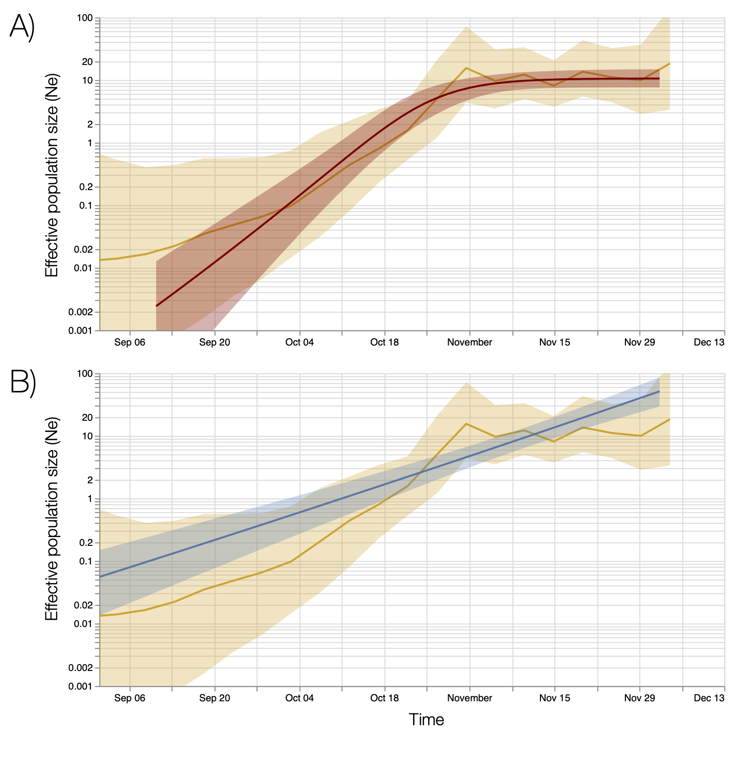
Figure S7 | Bayesian estimates of effective population size through time based on 776 genomes sampled between October and December 6. Top and bottom panels show estimates based on a Bayesian skygrid model overlaid with fits of different parametric models. A) Estimates based on a logistic growth model. B) Estimates from an exponential growth model.
References
- Preliminary genomic characterisation of an emergent SARS-CoV-2 lineage in the UK defined by a novel set of spike mutations. https://pando.tools/t/563 (2020).
- Chan, K. K., Tan, T. J. C., Narayanan, K. K. & Procko, E. An engineered decoy receptor for SARS-CoV-2 broadly binds protein S sequence variants. Cold Spring Harbor Laboratory 2020.10.18.344622 (2020) doi:10.1101/2020.10.18.344622.
- Starr, T. N. et al. Deep mutational scanning of SARS-CoV-2 receptor binding domain reveals constraints on folding and ACE2 binding. doi:10.1101/2020.06.17.157982.
- Gu, H. et al. Adaptation of SARS-CoV-2 in BALB/c mice for testing vaccine efficacy. Science 369, 1603–1607 (2020).
- Peacock, T. P., Goldhill, D. H., Zhou, J., Baillon, L. & Frise, R. The furin cleavage site of SARS-CoV-2 spike protein is a key determinant for transmission due to enhanced replication in airway cells. bioRxiv (2020).
- Bal, A. et al. Screening of the H69 and V70 deletions in the SARS-CoV-2 spike protein with a RT-PCR diagnosis assay reveals low prevalence in Lyon, France. medRxiv (2020).
- The COVID-19 Genomics UK (COG-UK) consortium. An integrated national scale SARS-CoV-2 genomic surveillance network. The Lancet Microbe 1, (2020).
- Volz, E. et al. Evaluating the Effects of SARS-CoV-2 Spike Mutation D614G on Transmissibility and Pathogenicity. Cell (2020) doi:10.1016/j.cell.2020.11.020.
- Flaxman, S. et al. Estimating the effects of non-pharmaceutical interventions on COVID-19 in Europe. Nature (2020) doi:10.1038/s41586-020-2405-7.
- Public Health England. Investigation of novel SARS-COV-2 variant: Variant of Concern 202012/01. Investigation of SARS-CoV-2 variants of concern: technical briefings - GOV.UK (2020).
- Mishra, S. et al. A COVID-19 Model for Local Authorities of the United Kingdom. medRxiv (2020).
- Volz, E. M. & Didelot, X. Modeling the growth and decline of pathogen effective population size provides insight into epidemic dynamics and drivers of antimicrobial resistance. Syst. Biol. (2018) doi:10.1093/sysbio/syy007.
- Hill, V. & Baele, G. Bayesian estimation of past population dynamics in BEAST 1.10 using the Skygrid coalescent model. Mol. Biol. Evol. (2019) doi:10.1093/molbev/msz172.
- Suchard, M. A. et al. Bayesian phylogenetic and phylodynamic data integration using BEAST 1.10. Virus Evol 4, vey016 (2018).
- Kemp, S., Harvey, W., Datir, R., Collier, D. & Ferreira, I. Recurrent emergence and transmission of a SARS-CoV-2 Spike deletion ΔH69/V70. bioRxiv (2020).
- du Plessis, L. et al. Establishment & lineage dynamics of the SARS-CoV-2 epidemic in the UK. medRxiv (2020).
- Hodcroft, E. B. et al. Emergence and spread of a SARS-CoV-2 variant through Europe in the summer of 2020. medRxiv (2020) doi:10.1101/2020.10.25.20219063.
- Minh, B. Q. et al. IQ-TREE 2: New Models and Efficient Methods for Phylogenetic Inference in the Genomic Era. Mol. Biol. Evol. 37, 1530–1534 (2020).
- Volz, E. M. & Frost, S. D. W. Scalable relaxed clock phylogenetic dating. Virus Evol 3, (2017).
- Wallinga, J. & Lipsitch, M. How generation intervals shape the relationship between growth rates and reproductive numbers. Proc. Biol. Sci. 274, 599–604 (2007).
- Lycett, S. J., Virgin, H. W., Telenti, A., Corti, D. & Robertson, D. L. The circulating SARS-CoV-2 spike variant N439K maintains fitness while evading antibody-mediated immunity. bioRxiv (2020).
- Trevor Hastie, R. T. Generalized Additive Models. Stat. Sci. 1, 297–310 (1986).
- Hastie, T., Tibshirani, R. & Friedman, J. H. The elements of statistical learning. (Springer, 2009).
- Rambaut, A. et al. A dynamic nomenclature proposal for SARS-CoV-2 to assist genomic epidemiology. Cold Spring Harbor Laboratory 2020.04.17.046086 (2020) doi:10.1101/2020.04.17.046086.
- Bhatt, S. et al. Semi-Mechanistic Bayesian Modeling of COVID-19 with Renewal Processes. arXiv [stat.AP] (2020).
- Bürkner, P.-C. brms: An R Package for Bayesian Multilevel Models Using Stan. Journal of Statistical Software, Articles 80, 1–28 (2017).