Early phylodynamics analysis of the COVID-19 epidemics in France
21-Apr-2020
Gonché Danesh, Baptiste Elie and Samuel Alizon
ETE Modelling group, MIVEGEC, CNRS, IRD, Université de Montpellier
Introduction
This report focuses on the COVID-19 epidemic in France using the SARS-Cov-2 genome data available from the GISAID - Global Initiative on Sharing All Influenza Data on April 10, 2020.
The first cases of COVID-19 were detected in France in Jan 2020, mostly from travelers, but they remained isolated. Incidence based on screening data only started to increase steadily in France on Feb 27. Limited measures were announced on Feb 28, but schools were closed from Mar 16 and a nationwide lockdown was implemented from Mar 17. On Apr 19, the prime minister E Philippe gave the first official estimate of the basic reproduction number (\mathcal{R}_0), which was 3.5. He also announced the temporal reproduction number had been dropped to 0.6.
We performed phylodynamics analyses using an exponential growth coalescent model in Beast 1.8.3 and a BDSKY model in Beast 2.3. Due to the low temporal signal in the data, we used molecular clocks with fixed values.
Here, we report results on the origin of the tree, the epidemic doubling time, the generation time and the temporal reproduction number \mathcal{R}(t).
Data used
On April 10, 194 sequences were available from samples originating from France. The vast majority of these sequences (94%) belong to the same clade labelled as A2 by nextstrain.
These sequences were aligned and cleaned using the Augur pipeline developed by nextstrain. One sequence was removed due to low qualityn, which led to a dataset of 186 sequences. The list is shown in Appendix.
We screened the dataset with RDP, which did not detect any recombination events.
The following graph shows the 186 sequences used, classified according to the date on which the sampling was carried out and the sampling region and France.
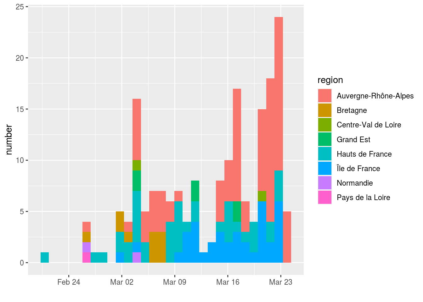
Some dates are over-represented in the dataset, which could bias the analysis. To correct for this, we sampled 7 sequences for each of the dates where more than 7 sequences were available. This was done twice to generate two datesets with 122 sequences (France122 and France122b).
To investigate temporal effects using the coalescent model, we created three other subsets of the France122 dataset:
-
France61-1 contains the 61 sequences sampled first (i.e. from Feb 21 to Mar 12),
-
France61-2 contains the 61 sequences sampled more recently (i.e. from Mar 12 to Mar 24),
-
France81 contains the 81 sequences sampled first (i.e. from Feb 21 to Mar 17).
With the exponential coalescent model (DT), we analysed the five subsets of data (Fra61-1, Fra61-2, Fra81, Fra122, and Fra122b), whereas we only report the most complete datasets (Fra122 and Fra122b) for the BDSKY model.
Results
Dating the TMRCA
We first report the estimation of the time to the most recent common ancestor (TMRCA) of all the sequences in the sample. Although this is the ancestor of the vast majority of the French sequences grouped in the A2 clade, it needs not be a French infection because there might have been multiple introductions of the epidemics in the country.
As pointed out by Louis Du Plessis, estimates of molecular clock should be treated with care. This is true in our case since we are analysing a small subset of the data. We therefore fix the default molecular clock to 8.8\cdot 10^{-4} substitutions/position/year as estimated by Andrew Rambaut on a larger phylogeny. We also investigated a low value (4.4\cdot 10^{-4} subst./pos./year) and a high value (13.2\cdot 10^{-4} subst./pos./year).
As expected, the molecular clock value directly affected the time to the most recent common ancestor. Note that the sampling of the 122 sequences amongst the 183 has a much smaller impact.

The table below shows the dates for a mean evolution rate value (8.8\cdot 10^{-4} subst/position/year).
| Model | Size | Most recent sample | lower bound (95%) | median | upper bound (95%) |
|---|---|---|---|---|---|
| Fix8.8-DT | 122 | 24 Mar 2020 | 19 Jan 2020 | 31 Jan 2020 | 09 Feb 2020 |
| Fix8.8-BDSKY | 122 | 24 Mar 2020 | 20 Jan 2020 | 31 Jan 2020 | 11 Feb 2020 |
| Fix8.8-DT | 122b | 24 Mar 2020 | 20 Jan 2020 | 02 Feb 2020 | 10 Feb 2020 |
| Fix13.2-DT | 122 | 24 Mar 2020 | 30 Jan 2020 | 08 Feb 2020 | 15 Feb 2020 |
| Fix4.4-DT | 122 | 24 Mar 2020 | 11 Dec 2019 | 01 Jan 2020 | 17 Jan 2020 |
Focusing on our largest datasets (with 122 sequences), our medium and high molecular clock assumptions date the common ancestor of the main clade regrouping the vast majority of the French sequences between mid-January and mid-February. This large interval is due to the rarity of “old” sequences (the first one collected in this clade dates from Feb 21) and on the fact that this clade averages the epidemics in several regions of France, which could have been seeded by independent introductions from outside France. Note that the “slow” molecular clock finds a root which seems very early given the data.
These dates are consistent with those obtained by Andrew Rambaut regarding the beginning of the epidemic in China, which is dated November 17, 2019 with a confidence interval between August 27 and December 19, 2020.
Doubling time
Using a coalescent model with exponential growth and serial sampling (Drummond et al 2002 Genetics), we can estimate the doubling time, which corresponds to the number of days for the epidemic to double in size. This parameter is key to calculate the basic reproduction number \mathcal{R}_0 (Wallinga & Lipsitch 2007 Proc B).
We show this doubling time for three of our datasets. Since the France122 dataset includes more recent sequences than France81, which itself includes more recent sequences than France61, our hypothesis is that we can detect variations in doubling time over the course of the epidemic.
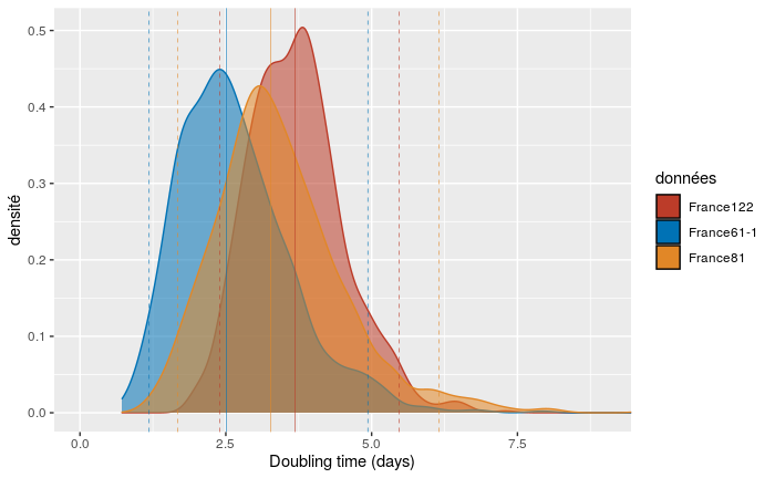
As can be seen in the figure, adding more recent sequence data leds to an increase in epidemic doubling time. Initially, with the first 61 sequences (which run from Feb 21 to Mar 12), the epidemic spreads rapidly, with a median doubly time of 2.5 days. With the addition of sequences sampled between March 12 and 17, the doubling time increases to 3.3 days. Finally, by adding sequences sampled between March 17 and 24, the doubling time rises to 3.7 days.
We also studied the effect of the molecular clock on the doubling time. For our realistic molecular clocks, the effect is limited: the median is 3.4 days assuming a high value for the molecular clock and 3.7 days for our default (medium) value.
The effect of tip sampling is much less pronounced. The low value of the molecular clock, which already led to unrealistic estimates for the origin of the epidemics, also led to a high median doubling time of 5.6 days. This is unrealistic given the incidence data in France, which indicates an exponential growth rate of 0.23 days ^{-1} which corresponds to a doubling time of 3 days.
In comparison, phylodynamic inferences made from data from China (with 86 genomes, Andrew Rambaut) found a median doubling time of about 7 days with a confidence interval between 4.7 and 16.3 days). The reason for the slower growth rate of the epidemic compared to ours is that we have focused on one rapidly expanding clade of the epidemic and neglected the smaller clades.
Duration of contagiousness
The birth-death skyline (BDSKY) model (Stadler et al 2013 Proc Nat Acad Sci USA) allows us to estimate of the duration of contagiousness and the reproduction number of the epidemic (i.e. the number of secondary infections caused by an infected host). The exponential growth coalescent model described above cannot distinguish between these two quantities.
Note that the BDSKY model requires more parameter values to be estimated. In addition, it is also necessary to estimate the sampling rate after Feb 21 (the date on which the oldest sequence was sampled) whereas the coalescent model assumes that this sampling is negligible.
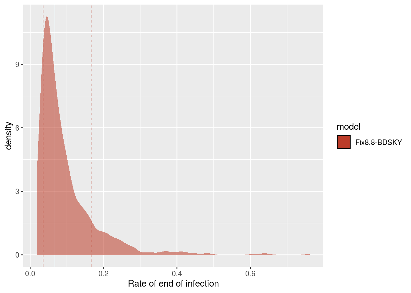
Posterior distribution for the rate of end of contagiousness estimated by Beast.
From this rate, we can obtain the duration of contagiousness, knowing that it is also necessary to account for the sampling rate because patients whose infections are sequenced can be assumed not to transmit the infection after this detection. The sampling rate is estimated at 0.093 days ^{-1} with a (wide) 95% confidence interval between 0.006 and 0.627 days ^{-1} (it is set to 0 prior to Feb 21).
The distribution of contagiousness durations is obtained by taking the inverse of the sum of the sampling rate and the contagiousness end rate (the inverse of a rate is a duration). The median of this distribution is 5.19 days and 95% of its values are between 1.52 and
8.52 days.
This result obtained using only dated sequences are consistent with those inferred using contact tracing. The latter measure serial intervals, which are used to approximate the length of the contagiousness period in the calculation of \mathcal{R}_0. For instance, Nishiura et al. (2020, Int J Infect Dis) find a distribution with a median of 4 days and a 95% confidence interval between 3.1 and 4.9 days.
Reproduction number
With the BDSKY model, we can estimate the effective reproductive number noted \mathcal{R}(t). Here, given the limited size of the dataset, we only divided the time into 3 intervals:
-
\mathcal{R}_1 estimates the temporal reproduction number before Feb 19,
-
\mathcal{R}_2 estimates the temporal reproduction number between Feb 19 and Mar 7,
-
\mathcal{R}_3 estimates the temporal reproduction number between Mar 7 and Mar 24.
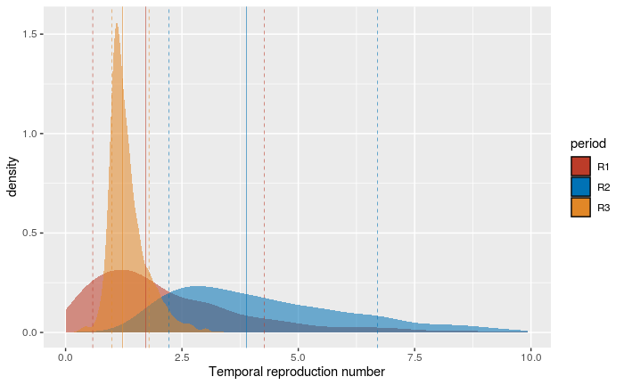
These results are very consistent with those obtained for the doubling time, even if the time periods are different. For the period before Feb 19, the estimate is the least accurate with values of \mathcal{R}_1 included at 95% between 0.13 and 7.01. This is consistent with the fact that the oldest sequence dates from February 21, while the tree root is estimated at the beginning of February. Over the second time period, rapid growth is detected since the values of \mathcal{R}_2 between 1.69 and 8.77. Finally, the most recent period after Mar 7 detects a slowing down of the epidemic with a \mathcal{R}_3 between 0.8 and 2.36.
Discussion and limits
Analysing SRAS-Cov-2 genome sequences with a known date of sampling allows to infer phylogenies of infections and to estimate epidemiological parameters. We performed this analysis based on the sequences representing the largest French clade within the phylogeny of all available SARS-Cov-2 sequences. This clade can be visualized on the nextstrain representation.
Before summarizing the results, we prefer to point out several limitations of our analysis:
-
the French clade we analyzed is in fact a European clade (and even international since many US sequences origate from it): although French most French sequences appear to be grouping into two subclades within this calde, it is possible that the variations in epidemic growth that we detect are more due to European than French control policies;
-
some French regions (e.g. Auvergne-Rhône-Alpes) are more represented than others, which could bias the analysis at the national level;
-
the molecular clock had to be set in this analysis because we do not have sufficient sampling during the month of February in France (the results with our average and high molecular clock are similar and consistent with the incidence data).
Despite these limitations, our results suggest a slowing down of the epidemic in France. Thus, by adding sequences sampled between March 12 and 24 to the phylogeny, the doubling time of the epidemic estimated by a exponential growth coalescent model increased by 48%. This slowdown more clearly detected using a birth death model via the temporal reproduction number \mathcal{R}(t): the median value increased from 3.88 before Mar 12 to a median value of 1.22 ater Mar 12. This is consistent with the implementation of strict control measures in France as of March 16. These variations and even these orders of magnitude are consistent with our estimates based on the time series of incidence of new hospitalizations and deaths in our Report 5.
Finally, the BDSKY model also provides us with an estimate of the duration of contagiousness, which is essential in the calculation of \mathcal{R}_0. The median value obtained (5.19 days) is consistent with some serial interval estimates for COVID-19 epidemics. To date, there is no estimate of the serial interval in France.
By increasing the number of SARS-CoV-2 genomic sequences from the French epidemic (and the number of people working on the subject), in particular sequences collected at the beginning of the epidemic, it would be possible to :
-
better estimate the date at which the epidemic took off in France,
-
better understand the spread between the different French regions,
-
estimate the number of virus introductions into the country.
Appendix
Priors
Exponential coalescent
| Parameter | Value |
|---|---|
| Molecular clock | fixed |
| Evolution model | GTR |
| kappa | lognormal[1, 1.25] |
| frequencies | uniform[0,1] |
| popsize | 1/x |
| growth rate | Gamma[0.001,1000] |
BDSKY
| Parameter | Value |
|---|---|
| Molecular clock | fixed |
| Evolution model | GTR |
| kappa | lognormal[1, 1.25] |
| frequencies | uniform[0,1] |
| Rate of end of infection | Unif(1.2,\infty) |
| Sampling rate | Beta(1,1) |
| Reprodution number | LogNorm(0,1.2) with max at 10 |
French sequence IDs
Click to see the whole table.
| Accession Number | Sampling Date | Region |
|:—|:---------:|:----:|:------![]()
| EPI_ISL_418415 | 2020-03-15 | Auvergne-Rhône-Alpes |
| EPI_ISL_418414 | 2020-03-15 | Auvergne-Rhône-Alpes |
| EPI_ISL_418413 | 2020-03-15 | Auvergne-Rhône-Alpes |
| EPI_ISL_418412 | 2020-03-15 | Auvergne-Rhône-Alpes |
| EPI_ISL_418419 | 2020-03-16 | Auvergne-Rhône-Alpes |
| EPI_ISL_418418 | 2020-03-16 | Auvergne-Rhône-Alpes |
| EPI_ISL_418417 | 2020-03-16 | Auvergne-Rhône-Alpes |
| EPI_ISL_418416 | 2020-03-16 | Auvergne-Rhône-Alpes |
| EPI_ISL_418431 | 2020-03-18 | Auvergne-Rhône-Alpes |
| EPI_ISL_418430 | 2020-03-18 | Auvergne-Rhône-Alpes |
| EPI_ISL_418422 | 2020-03-17 | Auvergne-Rhône-Alpes |
| EPI_ISL_418421 | 2020-03-17 | Auvergne-Rhône-Alpes |
| EPI_ISL_418420 | 2020-03-17 | Auvergne-Rhône-Alpes |
| EPI_ISL_418426 | 2020-03-17 | Auvergne-Rhône-Alpes |
| EPI_ISL_418425 | 2020-03-17 | Auvergne-Rhône-Alpes |
| EPI_ISL_418424 | 2020-03-17 | Auvergne-Rhône-Alpes |
| EPI_ISL_418423 | 2020-03-17 | Auvergne-Rhône-Alpes |
| EPI_ISL_418429 | 2020-03-18 | Auvergne-Rhône-Alpes |
| EPI_ISL_418428 | 2020-03-17 | Auvergne-Rhône-Alpes |
| EPI_ISL_418427 | 2020-03-17 | Auvergne-Rhône-Alpes |
| EPI_ISL_416750 | 2020-03-06 | Auvergne-Rhône-Alpes |
| EPI_ISL_416754 | 2020-03-06 | Auvergne-Rhône-Alpes |
| EPI_ISL_416751 | 2020-03-05 | Auvergne-Rhône-Alpes |
| EPI_ISL_416752 | 2020-03-04 | Auvergne-Rhône-Alpes |
| EPI_ISL_416757 | 2020-03-07 | Auvergne-Rhône-Alpes |
| EPI_ISL_416758 | 2020-03-08 | Auvergne-Rhône-Alpes |
| EPI_ISL_416756 | 2020-03-06 | Auvergne-Rhône-Alpes |
| EPI_ISL_416748 | 2020-03-04 | Auvergne-Rhône-Alpes |
| EPI_ISL_416749 | 2020-03-04 | Auvergne-Rhône-Alpes |
| EPI_ISL_416746 | 2020-03-03 | Auvergne-Rhône-Alpes |
| EPI_ISL_416747 | 2020-03-04 | Auvergne-Rhône-Alpes |
| EPI_ISL_416745 | 2020-03-10 | Auvergne-Rhône-Alpes |
| EPI_ISL_418231 | 2020-03-15 | Hauts de France |
| EPI_ISL_418230 | 2020-03-13 | Île de France |
| EPI_ISL_418235 | 2020-03-16 | Île de France |
| EPI_ISL_418234 | 2020-03-14 | Île de France |
| EPI_ISL_418233 | 2020-03-15 | Île de France |
| EPI_ISL_418232 | 2020-03-15 | Île de France |
| EPI_ISL_418239 | 2020-03-16 | Hauts de France |
| EPI_ISL_418238 | 2020-03-16 | Hauts de France |
| EPI_ISL_418237 | 2020-03-16 | Hauts de France |
| EPI_ISL_418236 | 2020-03-16 | Hauts de France |
| EPI_ISL_418220 | 2020-02-28 | Hauts de France |
| EPI_ISL_418224 | 2020-03-08 | Hauts de France |
| EPI_ISL_418223 | 2020-03-05 | Hauts de France |
| EPI_ISL_418222 | 2020-03-04 | Centre-Val de Loire |
| EPI_ISL_418221 | 2020-03-02 | Hauts de France |
| EPI_ISL_418228 | 2020-03-12 | Hauts de France |
| EPI_ISL_418227 | 2020-03-12 | Hauts de France |
| EPI_ISL_418226 | 2020-03-09 | Hauts de France |
| EPI_ISL_418225 | 2020-03-08 | Hauts de France |
| EPI_ISL_418229 | 2020-03-12 | Île de France |
| EPI_ISL_418240 | 2020-03-16 | Île de France |
| EPI_ISL_416493 | 2020-03-08 | Hauts de France |
| EPI_ISL_416496 | 2020-03-10 | Hauts de France |
| EPI_ISL_416497 | 2020-03-10 | Hauts de France |
| EPI_ISL_416494 | 2020-03-04 | Normandie |
| EPI_ISL_416495 | 2020-03-10 | Hauts de France |
| EPI_ISL_416498 | 2020-03-11 | Île de France |
| EPI_ISL_416499 | 2020-03-11 | Île de France |
| EPI_ISL_418219 | 2020-02-26 | Auvergne-Rhône-Alpes |
| EPI_ISL_418218 | 2020-02-21 | Hauts de France |
| EPI_ISL_414631 | 2020-03-04 | Grand Est |
| EPI_ISL_414630 | 2020-03-03 | Hauts de France |
| EPI_ISL_414633 | 2020-03-04 | Île de France |
| EPI_ISL_414632 | 2020-03-04 | Grand Est |
| EPI_ISL_414635 | 2020-03-04 | Hauts de France |
| EPI_ISL_414634 | 2020-03-04 | Hauts de France |
| EPI_ISL_414626 | 2020-02-29 | Hauts de France |
| EPI_ISL_414625 | 2020-02-26 | Pays de la Loire |
| EPI_ISL_414627 | 2020-03-02 | Hauts de France |
| EPI_ISL_414629 | 2020-03-03 | Hauts de France |
| EPI_ISL_414624 | 2020-02-26 | Normandie |
| EPI_ISL_414637 | 2020-03-04 | Hauts de France |
| EPI_ISL_414636 | 2020-03-04 | Hauts de France |
| EPI_ISL_414638 | 2020-03-04 | Hauts de France |
| EPI_ISL_420607 | 2020-03-23 | Auvergne-Rhône-Alpes |
| EPI_ISL_420606 | 2020-03-22 | Auvergne-Rhône-Alpes |
| EPI_ISL_420609 | 2020-03-23 | Auvergne-Rhône-Alpes |
| EPI_ISL_420608 | 2020-03-23 | Auvergne-Rhône-Alpes |
| EPI_ISL_420605 | 2020-03-22 | Auvergne-Rhône-Alpes |
| EPI_ISL_420604 | 2020-03-23 | Auvergne-Rhône-Alpes |
| EPI_ISL_420625 | 2020-03-24 | Auvergne-Rhône-Alpes |
| EPI_ISL_420624 | 2020-03-24 | Auvergne-Rhône-Alpes |
| EPI_ISL_420621 | 2020-03-24 | Auvergne-Rhône-Alpes |
| EPI_ISL_420620 | 2020-03-23 | Auvergne-Rhône-Alpes |
| EPI_ISL_420623 | 2020-03-24 | Auvergne-Rhône-Alpes |
| EPI_ISL_420622 | 2020-03-24 | Auvergne-Rhône-Alpes |
| EPI_ISL_420618 | 2020-03-23 | Auvergne-Rhône-Alpes |
| EPI_ISL_420617 | 2020-03-23 | Auvergne-Rhône-Alpes |
| EPI_ISL_420619 | 2020-03-23 | Auvergne-Rhône-Alpes |
| EPI_ISL_420614 | 2020-03-23 | Auvergne-Rhône-Alpes |
| EPI_ISL_420613 | 2020-03-23 | Auvergne-Rhône-Alpes |
| EPI_ISL_420616 | 2020-03-23 | Auvergne-Rhône-Alpes |
| EPI_ISL_420615 | 2020-03-23 | Auvergne-Rhône-Alpes |
| EPI_ISL_420610 | 2020-03-23 | Auvergne-Rhône-Alpes |
| EPI_ISL_420612 | 2020-03-23 | Auvergne-Rhône-Alpes |
| EPI_ISL_420611 | 2020-03-23 | Auvergne-Rhône-Alpes |
| EPI_ISL_416511 | 2020-03-07 | Bretagne |
| EPI_ISL_416512 | 2020-03-07 | Bretagne |
| EPI_ISL_416510 | 2020-03-06 | Bretagne |
| EPI_ISL_416513 | 2020-03-07 | Bretagne |
| EPI_ISL_416508 | 2020-03-06 | Bretagne |
| EPI_ISL_416509 | 2020-03-06 | Bretagne |
| EPI_ISL_416506 | 2020-03-03 | Bretagne |
| EPI_ISL_416500 | 2020-03-11 | Île de France |
| EPI_ISL_416501 | 2020-03-10 | Île de France |
| EPI_ISL_416504 | 2020-03-02 | Bretagne |
| EPI_ISL_416505 | 2020-03-02 | Bretagne |
| EPI_ISL_416502 | 2020-02-26 | Bretagne |
| EPI_ISL_417340 | 2020-03-07 | Auvergne-Rhône-Alpes |
| EPI_ISL_417333 | 2020-03-04 | Auvergne-Rhône-Alpes |
| EPI_ISL_417336 | 2020-03-06 | Auvergne-Rhône-Alpes |
| EPI_ISL_417337 | 2020-03-07 | Auvergne-Rhône-Alpes |
| EPI_ISL_417334 | 2020-03-04 | Auvergne-Rhône-Alpes |
| EPI_ISL_417338 | 2020-03-07 | Auvergne-Rhône-Alpes |
| EPI_ISL_417339 | 2020-03-08 | Auvergne-Rhône-Alpes |
| EPI_ISL_420056 | 2020-03-22 | Hauts de France |
| EPI_ISL_420055 | 2020-03-17 | Grand Est |
| EPI_ISL_420058 | 2020-03-20 | Île de France |
| EPI_ISL_420057 | 2020-03-22 | Hauts de France |
| EPI_ISL_420052 | 2020-03-20 | Île de France |
| EPI_ISL_420051 | 2020-03-19 | Île de France |
| EPI_ISL_420054 | 2020-03-20 | Île de France |
| EPI_ISL_420053 | 2020-03-19 | Hauts de France |
| EPI_ISL_420050 | 2020-03-19 | Hauts de France |
| EPI_ISL_420049 | 2020-03-19 | Hauts de France |
| EPI_ISL_420048 | 2020-03-18 | Île de France |
| EPI_ISL_420045 | 2020-03-17 | Grand Est |
| EPI_ISL_420044 | 2020-03-18 | Hauts de France |
| EPI_ISL_420047 | 2020-03-17 | Île de France |
| EPI_ISL_420046 | 2020-03-17 | Île de France |
| EPI_ISL_420041 | 2020-03-17 | Hauts de France |
| EPI_ISL_420040 | 2020-03-12 | Grand Est |
| EPI_ISL_420043 | 2020-03-18 | Île de France |
| EPI_ISL_420042 | 2020-03-17 | Île de France |
| EPI_ISL_420038 | 2020-03-17 | Auvergne-Rhône-Alpes |
| EPI_ISL_420039 | 2020-03-12 | Grand Est |
| EPI_ISL_420063 | 2020-03-22 | Île de France |
| EPI_ISL_420062 | 2020-03-22 | Île de France |
| EPI_ISL_420064 | 2020-03-23 | Île de France |
| EPI_ISL_420061 | 2020-03-23 | Île de France |
| EPI_ISL_420060 | 2020-03-20 | Île de France |
| EPI_ISL_420059 | 2020-03-21 | Île de France |
| EPI_ISL_421513 | 2020-03-23 | Île de France |
| EPI_ISL_421514 | 2020-03-20 | Centre-Val de Loire |
| EPI_ISL_421511 | 2020-03-23 | Hauts de France |
| EPI_ISL_421512 | 2020-03-23 | Île de France |
| EPI_ISL_421510 | 2020-03-23 | Hauts de France |
| EPI_ISL_421508 | 2020-03-23 | Île de France |
| EPI_ISL_421509 | 2020-03-23 | Hauts de France |
| EPI_ISL_421506 | 2020-03-21 | Île de France |
| EPI_ISL_421507 | 2020-03-23 | Île de France |
| EPI_ISL_421504 | 2020-03-14 | Île de France |
| EPI_ISL_421505 | 2020-03-15 | Île de France |
| EPI_ISL_421502 | 2020-03-12 | Île de France |
| EPI_ISL_421503 | 2020-03-12 | Île de France |
| EPI_ISL_421500 | 2020-03-11 | Hauts de France |
| EPI_ISL_421501 | 2020-03-12 | Île de France |
| EPI_ISL_415650 | 2020-03-02 | Île de France |
| EPI_ISL_415652 | 2020-03-05 | Auvergne-Rhône-Alpes |
| EPI_ISL_415651 | 2020-03-05 | Auvergne-Rhône-Alpes |
| EPI_ISL_415654 | 2020-03-09 | Hauts de France |
| EPI_ISL_415653 | 2020-03-08 | Hauts de France |
| EPI_ISL_415649 | 2020-03-05 | Hauts de France |
| EPI_ISL_419169 | 2020-03-21 | Auvergne-Rhône-Alpes |
| EPI_ISL_419168 | 2020-03-17 | Auvergne-Rhône-Alpes |
| EPI_ISL_419188 | 2020-03-22 | Auvergne-Rhône-Alpes |
| EPI_ISL_419187 | 2020-03-22 | Auvergne-Rhône-Alpes |
| EPI_ISL_419186 | 2020-03-22 | Auvergne-Rhône-Alpes |
| EPI_ISL_419185 | 2020-03-22 | Auvergne-Rhône-Alpes |
| EPI_ISL_419180 | 2020-03-22 | Auvergne-Rhône-Alpes |
| EPI_ISL_419184 | 2020-03-22 | Auvergne-Rhône-Alpes |
| EPI_ISL_419183 | 2020-03-22 | Auvergne-Rhône-Alpes |
| EPI_ISL_419182 | 2020-03-22 | Auvergne-Rhône-Alpes |
| EPI_ISL_419181 | 2020-03-22 | Auvergne-Rhône-Alpes |
| EPI_ISL_419177 | 2020-03-22 | Auvergne-Rhône-Alpes |
| EPI_ISL_419176 | 2020-03-21 | Auvergne-Rhône-Alpes |
| EPI_ISL_419175 | 2020-03-21 | Auvergne-Rhône-Alpes |
| EPI_ISL_419174 | 2020-03-20 | Auvergne-Rhône-Alpes |
| EPI_ISL_419179 | 2020-03-22 | Auvergne-Rhône-Alpes |
| EPI_ISL_419178 | 2020-03-22 | Auvergne-Rhône-Alpes |
| EPI_ISL_419173 | 2020-03-21 | Auvergne-Rhône-Alpes |
| EPI_ISL_419172 | 2020-03-21 | Auvergne-Rhône-Alpes |
| EPI_ISL_419171 | 2020-03-21 | Auvergne-Rhône-Alpes |
| EPI_ISL_419170 | 2020-03-21 | Auvergne-Rhône-Alpes |
Software used
-
Sequence alignment was obtained through the Augur pipeline developed by nextstrain.
-
The choice of the surrogate genetic model was made using SMS software.
-
The maximum likelihood phylogeny was inferred using PhyML.
-
The search for temporal signal of molecular evolution was carried out using the software TempEst.
-
The phylodynamic analyses were performed using version 1.8.3 of the software Beast and version 2.3 of the software Beast2.
-
Additional manipulations were performed in R using the ape package.
Sources and acknowledgements
-
DNA sequence data have been provided by several international laboratories and made available through GISAID - Global Initiative on Sharing All Influenza Data.
-
We thank the patients, nurses, doctors and all the French laboratories who made this work possible by generating and sharing the virus genome sequences.
-
The authors thank the high-performance computer itrop (platform South Green) of the IRD of Montpellier for the provision of the high-performance computing resources, which contributed to the results presented in this work (more details on bioinfo.ird.fr).
-
The ETE modelling team is composed of Samuel Alizon, Thomas Bénéteau, Marc Choisy, Gonché Danesh, Ramsès Djidjou-Demasse, Baptiste Elie, Yannis Michalakis, Bastien Reyné, Quentin Richard, Christian Selinger, Mircea T. Sofonea.
-
Contribution to this work:
-
conception of the work: the whole team
-
carrying out analyses: GD, BE and SA
-
report writing: SA
-
contacts: [email protected], [email protected], [email protected]
-
approval: the whole team
-
-

This work is made available under the terms of the Creative Commons Attribution-Noncommercial 4.0 International License.