This post has been updated with new data here:
http://virological.org/t/phylodynamic-analysis-44-genomes-29-jan-2020/356/2
This post has been updated with new data here:
http://virological.org/t/phylodynamic-analysis-44-genomes-29-jan-2020/356/2
Temporal signal of nCoV-2019 based on 30 genomes
January 29, 2020
Louis du Plessis, University of Oxford
[email protected]
This is a brief report investigating the molecular clock signal in the sequenced nCoV-2019 genomes (based on 30 publicly shared genome sequences). This is still work in progress and is for information purposes only. Estimates of the clock rate and TMRCA should not be considered reliable and all estimates should be considered based on their intervals and not point values. Skip to the end for my conclusions and recommendations.
All of the caveats above also hold for the dataset and analyses presented below.
I used the 30 genome (29,903 bp) dataset used by Kristian Andersen (http://virological.org/t/clock-and-tmrca-based-on-27-genomes/347/5) from 27 January. See Kristian’s post for genome acknowledgements and availability. A few more genomes are available now (see above).
| Id | Accession | Location | Collection date | Ambiguous sites | Gaps |
|---|---|---|---|---|---|
| EPI_ISL_402123 | - | Wuhan | 2019-12-24 | 0 | 4 |
| CNA0007332 | - | Wuhan | 2019-12-26 | 0 | 37 |
| EPI_ISL_402125 | - | Wuhan | 2019-12-26 | 0 | 0 |
| EPI_ISL_402128 | - | Wuhan | 2019-12-30 | 0 | 51 |
| EPI_ISL_402132 | - | Wuhan | 2019-12-30 | 0 | 55 |
| EPI_ISL_402130 | - | Wuhan | 2019-12-30 | 0 | 46 |
| EPI_ISL_402129 | - | Wuhan | 2019-12-30 | 0 | 49 |
| EPI_ISL_402127 | - | Wuhan | 2019-12-30 | 0 | 59 |
| EPI_ISL_403930 | - | Wuhan | 2019-12-30 | 0 | 4 |
| EPI_ISL_402119 | - | Wuhan | 2019-12-30 | 0 | 12 |
| EPI_ISL_402124 | - | Wuhan | 2019-12-30 | 0 | 12 |
| EPI_ISL_402121 | - | Wuhan | 2019-12-30 | 2 | 12 |
| EPI_ISL_403929 | - | Wuhan | 2019-12-30 | 0 | 13 |
| EPI_ISL_403931 | - | Wuhan | 2019-12-30 | 6 | 14 |
| EPI_ISL_402120 | - | Wuhan | 2020-01-01 | 96 | 116 |
| CNA0007334 | - | Wuhan | 2020-01-01 | 0 | 35 |
| CNA0007335 | - | Wuhan | 2020-01-05 | 0 | 32 |
| EPI_ISL_403962 | - | Thailand | 2020-01-08 | 0 | 55 |
| EPI_ISL_403963 | - | Thailand | 2020-01-13 | 0 | 44 |
| aGenbank | MN975262 | Guangdong | 2020-01-14 | 0 | 12 |
| EPI_ISL_403932 | MN938384 | Guangdong | 2020-01-14 | 0 | 58 |
| EPI_ISL_403933 | - | Guangdong | 2020-01-15 | 0 | 58 |
| EPI_ISL_403935 | - | Guangdong | 2020-01-15 | 0 | 58 |
| EPI_ISL_403934 | - | Guangdong | 2020-01-15 | 0 | 58 |
| EPI_ISL_404227 | - | Zhejiang | 2020-01-16 | 1 | 64 |
| EPI_ISL_403936 | - | Guangdong | 2020-01-17 | 0 | 58 |
| EPI_ISL_404228 | - | Zhejiang | 2020-01-17 | 0 | 44 |
| EPI_ISL_403937 | - | Guangdong | 2020-01-18 | 0 | 58 |
| EPI_ISL_404895 | MN985325 | USA | 2020-01-19 | 0 | 21 |
| EPI_ISL_404253 | MN988713 | USA | 2020-01-21 | 2 | 21 |
Because the number of sites in the alignment with ambiguous nucleotides or indels far exceeds the number of fully resolved sites I investigated the possibility that those sites could be responsible for the clock signal in the dataset.
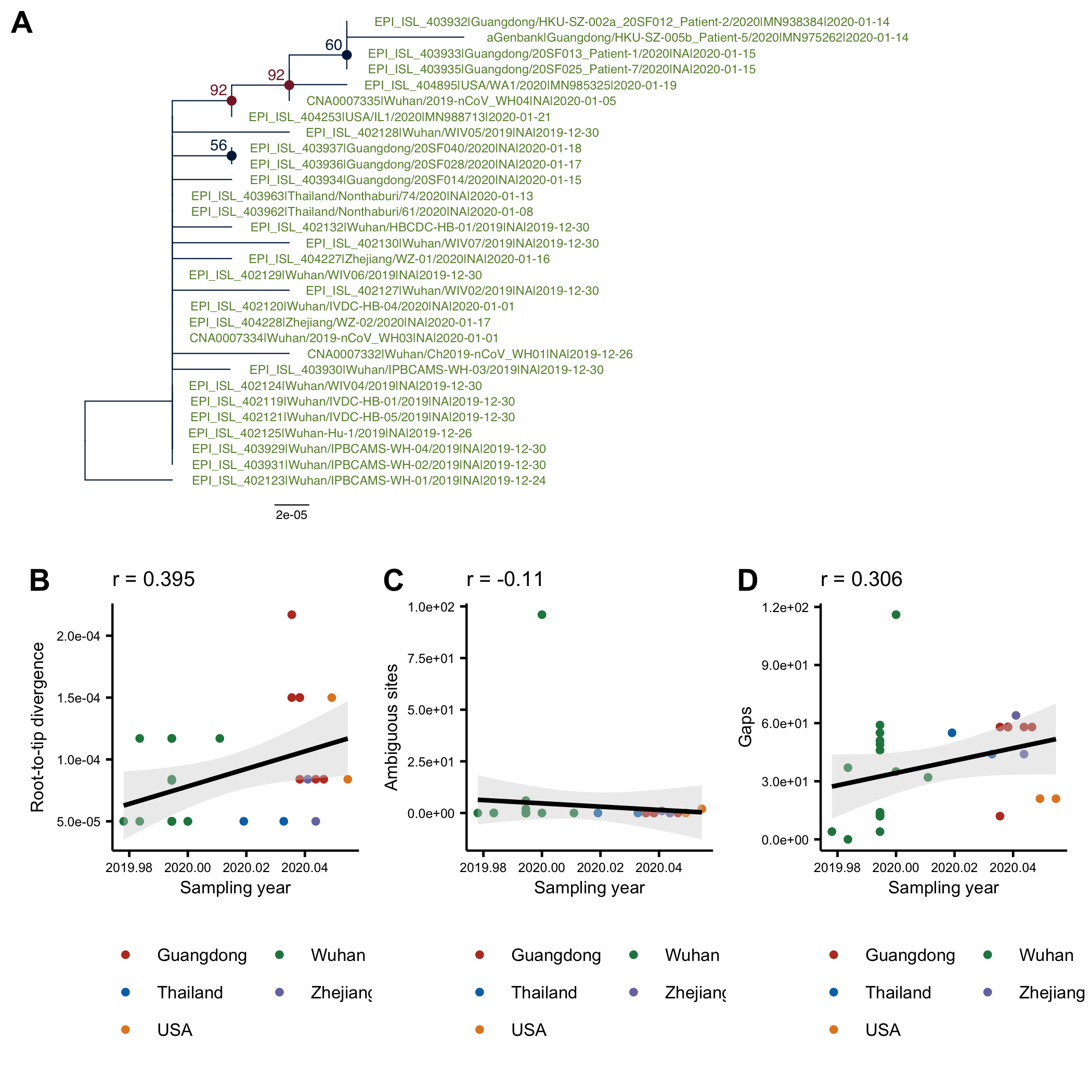
The phylogenetic tree (genetic distance) for the 30-genome alignment is shown Fig1A. The tree was computed in PhyML and is arbitrarily rooted using the oldest sequence. On Fig1B it can be seen that there is a positive correlation between the root-to-tip distance and the collection date, which is indicative of clock-like evolution (although the residuals are large). Although there is no association between the number of ambiguous sites and the collection date, the correlation between the number of indels/gaps and collection date is almost as high as between the root-to-tip distance and collection date.
Figure 1: (A) ML tree of the full alignment rooted using the oldest sequence. (B) Root-to-tip distance in the ML tree plotted against sampling date. C) Number of ambiguous sites in a sequence plotted against the sampling date. (D) Number of gaps in a sequence plotted against the sampling date.
To control for this association I created two more alignments:
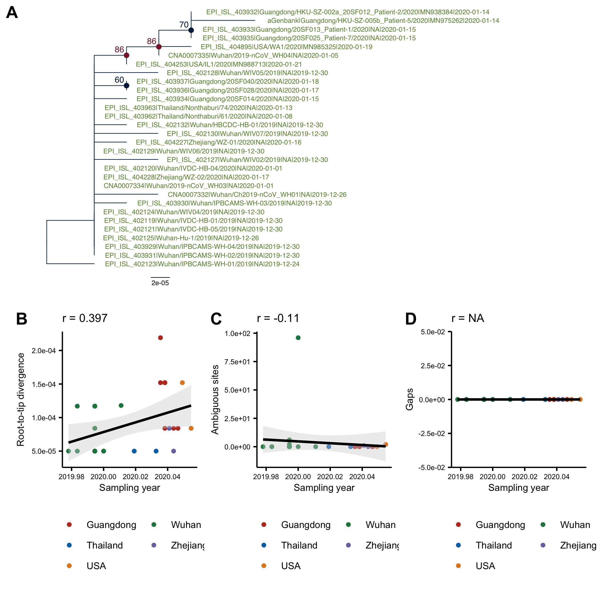
The tree on the trimmed alignment (Fig 2A) is almost identical to the tree on the full alignment (Fig1A). There is still a correlation between the root-to-tip distance and the collection date (Fig2B), but no longer any correlation with the numbers of ambiguous sites or gaps.
Figure 2: (A) ML tree of the trimmed alignment rooted using the oldest sequence. (B) Root-to-tip distance in the ML tree plotted against sampling date. C) Number of ambiguous sites in a sequence plotted against the sampling date. (D) Number of gaps in a sequence plotted against the sampling date.
The tree on the fully resolved alignment (Fig3A) looks different because of two sites in EPI_ISL_404253 that are labelled Y (pyramidine). There are also mutations for other genomes at these two sites which are informative for the tree structure. When these two sites are included the tree is almost identical to the previous two trees. There is still a positive association between root-to-tip distance and collection date, although it is smaller than on the full or trimmed alignments.
Figure 3: (A) ML tree of the fully resolved alignment rooted using the oldest sequence. (B) Root-to-tip distance in the ML tree plotted against sampling date. C) Number of ambiguous sites in a sequence plotted against the sampling date. (D) Number of gaps in a sequence plotted against the sampling date.
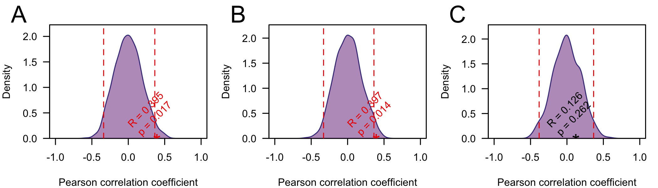
To test if the correlations between the root-to-tip distance and collection date are significant I performed a simple date shuffling analysis (as in Murray et al. (2015)). Briefly, to assess the significance of the correlations I permute the sampling dates across genome sequences (in the tree) and us the Pearson correlation coefficient as a test statistic. I performed 1000 replicates and calculated the p-value as the proportion of replicates with a correlation coefficient greater than or equal to the truth (using unpermuted collection dates) (Fig4). Using this test the correlation was significant (p < 0.05) on the full and trimmed alignments. On the fully resolved alignment it was not significant, but this is not suprising, since the tree lacks the full structure.
Figure 4: Null distribution of the Pearson correlation coefficient between root-to-tip distance and sampling date) for the full alignment (A) the alignment with ends trimmed (B) and the fully resolved alignment C). The dashed lines indicate 2.5 and 97.5 quantiles of the distribution and the star indicates the correlation coefficient using the true (unpermuted) sampling dates. The p-value is the proportion of replicates with the test statistic (Pearson correlation coefficient) greater than or equal to the true value.
I used BEASTv2.6 (Bouckaert et al. (2019)) to estimate the clock rate and the TMRCA on the full and trimmed alignments under an HKY subsitution model and a strict clock. I used three demographic models:
This was mostly to see if different demographic models lead to different estimates or mixing and not to infer anything about the population dynamics [more on this at the end]. I used a uniform prior on [0, 1E-2] on the clock rate. This was not meant to be an uninformative prior, but was to test if posterior estimates are informed mostly by the data or the prior choice. I used the default priors for all other model parameters. I ran 3 chains/model for 50 million states, sampling every 5000 states. For each model all 3 chains converged to the same posterior (discarding 10% of chains as burn-in).
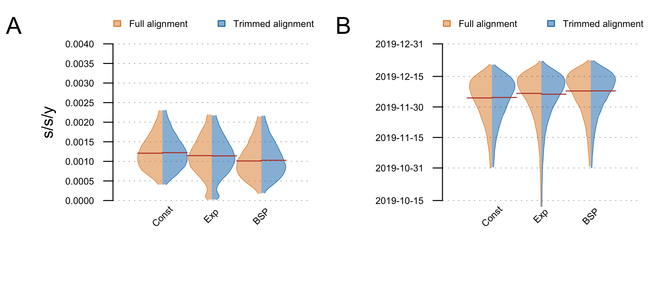
The posterior clock-rate and TMRCA estimates are shown in Fig5. Estimates are nearly identical on the full and trimmed alignment. The demographic model does not make a big difference to the estimates, although the exponential growth coalescent has some support for very low clock rates (resulting in an older TMRCA). These estimates are very similar to the ones reported by Andrew (above) and Kristian Andersen (http://virological.org/t/clock-and-tmrca-based-on-27-genomes/347/5).
Figure 5: Posterior distributions of the clock rate (A) and TMRCA (B) estimated on the full and trimmed alignments under different demographic models (tree-priors). The distributions are truncated at the upper and lower limits of the 95% HPD interval and the red lines indicate the median estimates.
I also sampled from the prior (on the full alignment), but these runs did not converge (specifically, the demographic model parameters did not mix). When sampling from the prior the clock rate recovered the prior I set (Uniform(0,1E-2)), showing that the posterior clock rate estimates are indeed different to the prior.
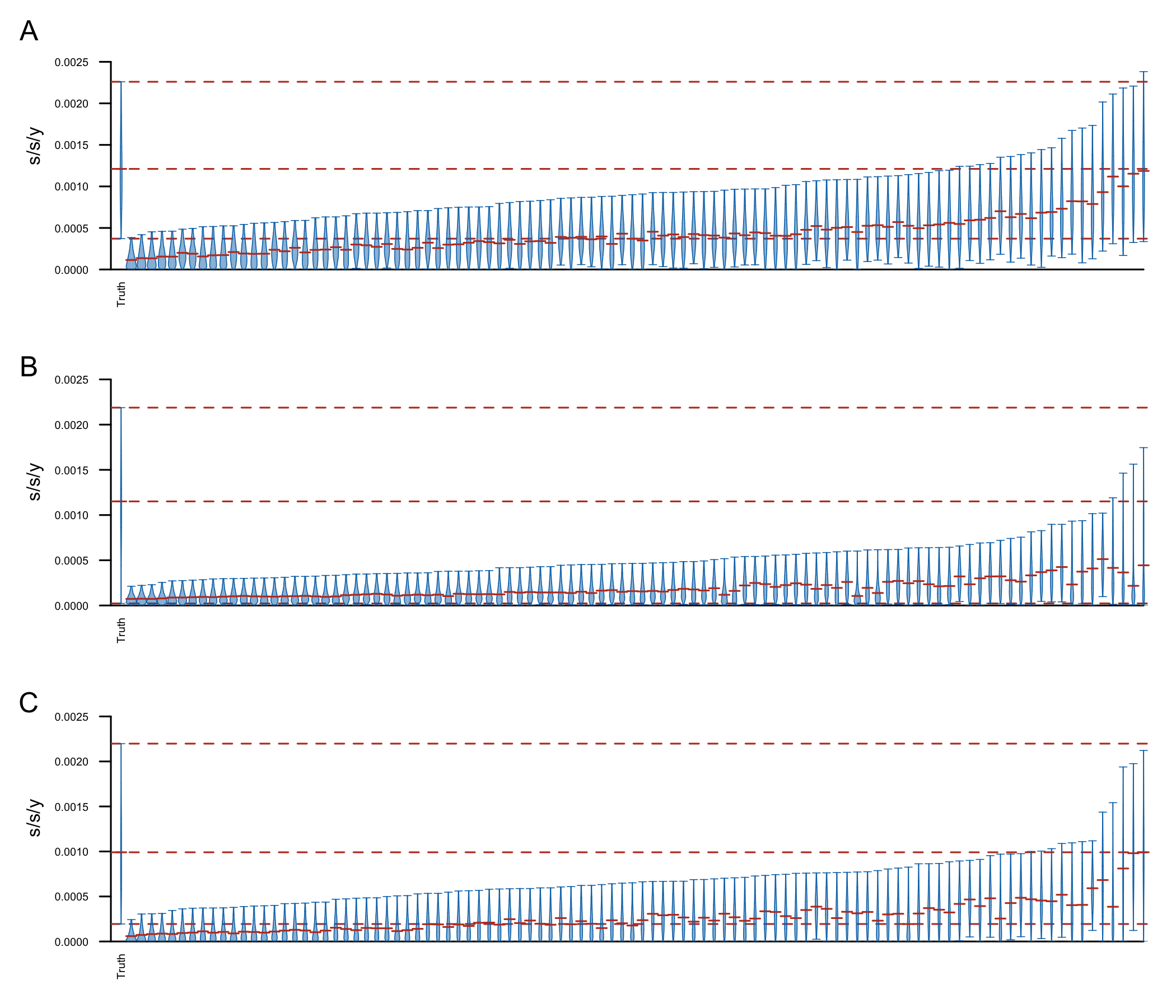
To confirm that the clock signal is significant I performed a Bayesian date randomization test (Duchêne et al. (2015)), permuting sampling dates across genomes and repeating the above analyses (100 replicates). The results are shown in Fig6. Although the clock rate estimated using the true sampling dates is in general faster than the rate estimated on the shuffled dates, some of the replicates have 95% HPD intervals including the median clock rate estimate, and a few replicates resulted in very similar estimates (to estimates using the true sampling dates). This could be because of a few reasons:
**Figure 6: ** Date shuffling analyses performed under a constant size (A), exponential growth (B) and Bayesian skyline plot (C) coalescent tree prior and a strict clock model. The plot shows the posterior distributions for the clock rate, truncated at the upper and lower limits of the 95% HPD interval. Horizontal red lines indicate the medians of the posterior distributions. The red dashed lines indicate the median and upper and lower limits of the 95% HPD interval of the clock rate inferred under the true sampling dates.
The temporal horizon (the average time taken to accumulate a mutation) for coronaviruses is about 1-2 weeks (see Fig6 in Dudas et al. (2019)). With a sampling period of only about 1 month between the oldest and most recent sequences there won’t be a very strong molecular clock signal in the data (yet). However, the dataset already shows some signal and the signal is coming from the mutations and not ambiguous sites or gaps/indels. Estimates of the clock rate and TMRCA appear to be relatively robust (if wide), however I’m not fully convinced that the clock signal is significant at this point.
My recommendation: Proceed with caution. Clock rate and TMRCA estimates are likely to contain the truth, but will be uncertain (wide HPDs). Do not rely on point estimates since median and mean estimates are likely to be biased. Remember that the TMRCA is for the sample and not the entire outbreak!
At this point in time I would not trust any conclusions drawn from a demographic model that is informed only by the sampled tree / genomes. If anything, fitting a demographic model to this dataset will show a decrease in effective population size (or R), simply because most of the coalescences are close to the root (in the big polytomy). This would suggest large growth close to the root, followed by slower growth or declining population size, but this reasoning is wrong because it doesn’t take the extremely biased sampling up to this point into account. Several of the Wuhan sequences in the tree were likely close contacts and sampled around the same time (so they were not drawn at random from a well-mixed population). The same goes for the family clusters of 3 identical sequences from Shenzhen and 2 identical sequences from Zhuhai. So not only do you have big changes in the sampling rate over time, but even over a short time period some samples are preferentially drawn because of their association with other cases (e.g. family members or work colleagues). It’s also likely that there is strong population structure in the dataset, since most of the older genomes are from Wuhan and the more recent genome sequences are not from Hubei, so there may be some source/sink dynamics at play here.
Another issue with demographic models is that almost all available tools are only for strictly bifurcating trees, but the genetic distance tree has several polytomies on it. BEAST will resolve the polytomies using the sampling dates where possible, but some are still likely to be arbitrarily resolved. The result would be to pull coalescent times closer to the present than the truth and since most demographic models rely on the timing of coalescences as their main source of information this could lead to biased estimates.
My recommendation: Until more time has passed the demographic model is not likely to be informative. Since the demographic model may lead to biased parameter estimates it’s a good idea to try a few different models and ensure that estimates are robust to the demographic model used. Do not draw conclusions about the effective population size, serial interval or reproductive number from demographic models informed only by genomic data.
Murray, Gemma G. R., Fang Wang, Ewan M. Harrison, Gavin K. Paterson, Alison E. Mather, Simon R. Harris, Mark A. Holmes, Andrew Rambaut, and John J. Welch. 2015. “The Effect of Genetic Structure on Molecular Dating and Tests for Temporal Signal.” Methods in Ecology and Evolution, 80–89.
Bouckaert, Remco, Timothy G. Vaughan, Joëlle Barido-Sottani, Sebastián Duchêne, Mathieu Four- ment, Alexandra Gavryushkina, Joseph Heled, et al. 2019. “BEAST 2.5: An Advanced Software Platform for Bayesian Evolutionary Analysis.” PLOS Computational Biology 15 (4): e1006650. doi:10.1371/journal.pcbi.1006650.
Duchêne, Sebastián, David Duchêne, Edward C. Holmes, and Simon Y. W. Ho. 2015. “The Performance of the Date-Randomization Test in Phylogenetic Analyses of Time-Structured Virus Data.” Molecular Biology and Evolution 32 (7): 1895–1906. doi:10.1093/molbev/msv056.
Dudas, Gytis, and Trevor Bedford. 2019. “The Ability of Single Genes Vs Full Genomes to Resolve Time and Space in Outbreak Analysis.” BMC Evolutionary Biology 19 (1): 232. doi:10.1186/s12862-019-1567-0.