Preliminary analysis of SARS-CoV-2 importation & establishment of UK transmission lineages
Methods and Appendices
8th June 2020
Oliver Pybus1 & Andrew Rambaut2 with Louis du Plessis1, Alexander E Zarebski1, Moritz U G Kraemer1, Jayna Raghwani1, Bernardo Gutiérrez1, Verity Hill2, John McCrone2, Rachel Colquhoun2, Ben Jackson2, Áine O’Toole2, Jordan Ashworth2, on behalf of the COG-UK consortium3
1 University of Oxford, 2 University of Edinburgh, 3 https://www.cogconsortium.uk
Summary of Methods
UK transmission lineages were identified from SARS-CoV-2 genomes generated by the COG-UK consortium and genomics teams in other countries worldwide. Virus genomes used in this study are publicly available from https://www.cogconsortium.uk/data and https://www.gisaid.org.
All available virus genome sequences with appropriate metadata as of 22nd May 2020 were collated and aligned. Large-scale phylogenetic trees were estimated separately using IQTree v1.6.12 for the following global lineages: A (n=2056), B (n=3330), B.1 (n=7505), B.1.X (n=8408), B.1.Y.X (n=4157), and B.2 (n=2943). UK transmission lineages within these large-scale trees were identified using a parsimony reconstruction of a two-state character (UK, non-UK). Many internal phylogeny nodes are polytomies comprising multiply sequenced identical genomes. If the genomes at such nodes had both UK and non-UK states, then the polytomy character state was conservatively reconstructed as non-UK. The UK genomes that exist at such polytomies were labelled as singletons. This approach aims to be conservative, i.e. it will likely underestimate the number of detected UK transmission lineages. The approach used here is specifically designed to identify UK transmission lineages descended from distinct introductions and is different from the “UK lineage” designation used within the COG-UK consortium for other purposes.
Each of these large-scale phylogenies was converted into a time-scaled tree by applying an externally-estimated posterior distribution of the rate of SARS-CoV-2 genome evolution (see below). The posterior rate had a mean of 9.41×10⁻⁴ nucleotide substitutions per site per year and a standard deviation of 4.99×10⁻⁵. This rate was estimated from an alignment of 710 SARS-CoV-2 genomes sampled longitudinally through time using an HKY substitution model, a strict molecular clock model, and a skygrid coalescent prior, as implemented in BEAST 1.10. The conversion to time-scaled trees was performed using the strict molecular clock approach implemented in treedater (minimum branch length = 0.01 days). Molecular clock estimation was replicated 150 times for each large-scale phylogenetic tree, using 150 random resolutions of polytomies and 150 random rates drawn from the posterior distribution described above. The resulting distribution of TMRCA values therefore incorporates uncertainty in the estimated clock rate and polytomy resolution.
To estimate temporal trends in SARS-CoV-2 importation intensity we sought information on (i) the number of travellers entering the UK from each source country (comprising both British nationals and resident and visiting citizens of other countries) and (ii) the prevalence (i.e. number of infectious individuals) in each source country on each day.
Estimates for item (i) were generated by combining multiple data sources. The first source was a Home Office report providing numbers of inbound travellers arriving in the UK by air on each day during Jan-Apr 20209. The second source was the percentage of inbound flight journeys to the UK that start from each country. These percentages are calculated from IATA data on a monthly basis, for January, February and March 2020. The proportions of inbound passengers from each country vary little between countries through time, so the percentages for March were extrapolated to April (for which no data is available). We combined these two data sources to estimate the number of air passenger arrivals in the UK from each country on each day. Third, we augmented the air passenger numbers with estimated numbers of travellers arriving per day by short-sea ferry and rail. The numbers of ferry passengers from France, Netherlands and the Republic of Ireland, and the number of Eurotunnel vehicle movements, were obtained from publicly available monthly records. Inbound rail travellers from France and Belgium were estimated from historical data and adjusted as far as possible for post-pandemic reduction in travel. Estimates of short-sea ferry arrivals in April, and of rail arrivals on all months, are less certain than those for travellers by air. Note, we have not incorporated estimates of land-border movements with the Republic of Ireland.
Estimates for item (ii) were obtained by back-extrapolating time series of cumulative deaths due to COVID-19 in each country. Cumulative death numbers were extracted from the Johns Hopkins University database (containing data from January 23rd to May 30th). Time series of reported deaths related to COVID-19 reported deaths were used rather than confirmed cases as we are primarily interested in temporal dynamics rather than absolute values, and counts of deaths are believed to be less sensitive to changes in case definition and the level of surveillance. The difference in the number of cumulative cases on each day was used as the number of deaths on that day, truncated as zero for days where the cumulative value decreased (due to changes in reported numbers). On 17th April, 1290 additional deaths were added to the cumulative number of deaths in China that had occurred since the beginning of the epidemic but were not previously part of the database. Without a reliable way to distribute them across the time series, the count on this day was set to the same value as the preceding and subsequent days: zero. Estimates of the time after infection that an individual becomes infectious and experiences symptoms, the infectious duration, and the time between symptom onset and death (among those who will die from COVID-19) were taken from peer-reviewed sources10. Specifically we assumed an individual becomes infectious 3 days after being infected, symptoms begin 2 days later, the infectious period ends 5 days after that, and for those who will die, they do so 18 days after the onset of symptoms. Since the numbers of deaths is large, the variation in these timings among individuals will be averaged out and is not considered. Accounting for the amount of time each fatal case was infectious and how many fatalities there were on each day, we estimated the total number of infectious individuals (who would subsequently be reported as having died due to COVID-19) on each day. We estimated the total number of infectious individuals on each day as the number of infectious individuals (who would eventually die) on that day multiplied by the reciprocal of the infection fatality rate, which was set to be 1% (a value broadly consistent with those found in the literature for China, France, and passengers aboard the Diamond Princess; Verity et al (2020), Russel et al (2020), Roques et al (2020)). However, the main results presented here are invariant to the value of this scalar. Due to right censoring of the time series (i.e. recent dates do not incorporate those who will, but have not yet, died), the last 25 days were ignored and we only consider data up to May 5th.
To estimate the importation lag, the number of transmission lineage TMRCAs on each day was modelled as a constant fraction of the total number of importation events on each day up until then, where the propensity of a new importation to begin a transmission lineage is Poisson-weighted by how long ago it arrived. For example, for an average lag of 2 days, a transmission lineage whose TMRCA is on Friday could be due to an importation event on Monday or Tuesday, but is more likely to be due to an importation event on Wednesday. Due to the statistical properties of the TMRCA of a random sample from a subtree, the importation lag is expected to be longer for smaller transmission lineages. To account for this we fitted one lag for transmission lineages with 2-5 genomes (estimated to be 11.9 days), one lag for lineages with 6-15 genomes (9.4 days) and another lag for lineages >15 genomes (4.2 days).
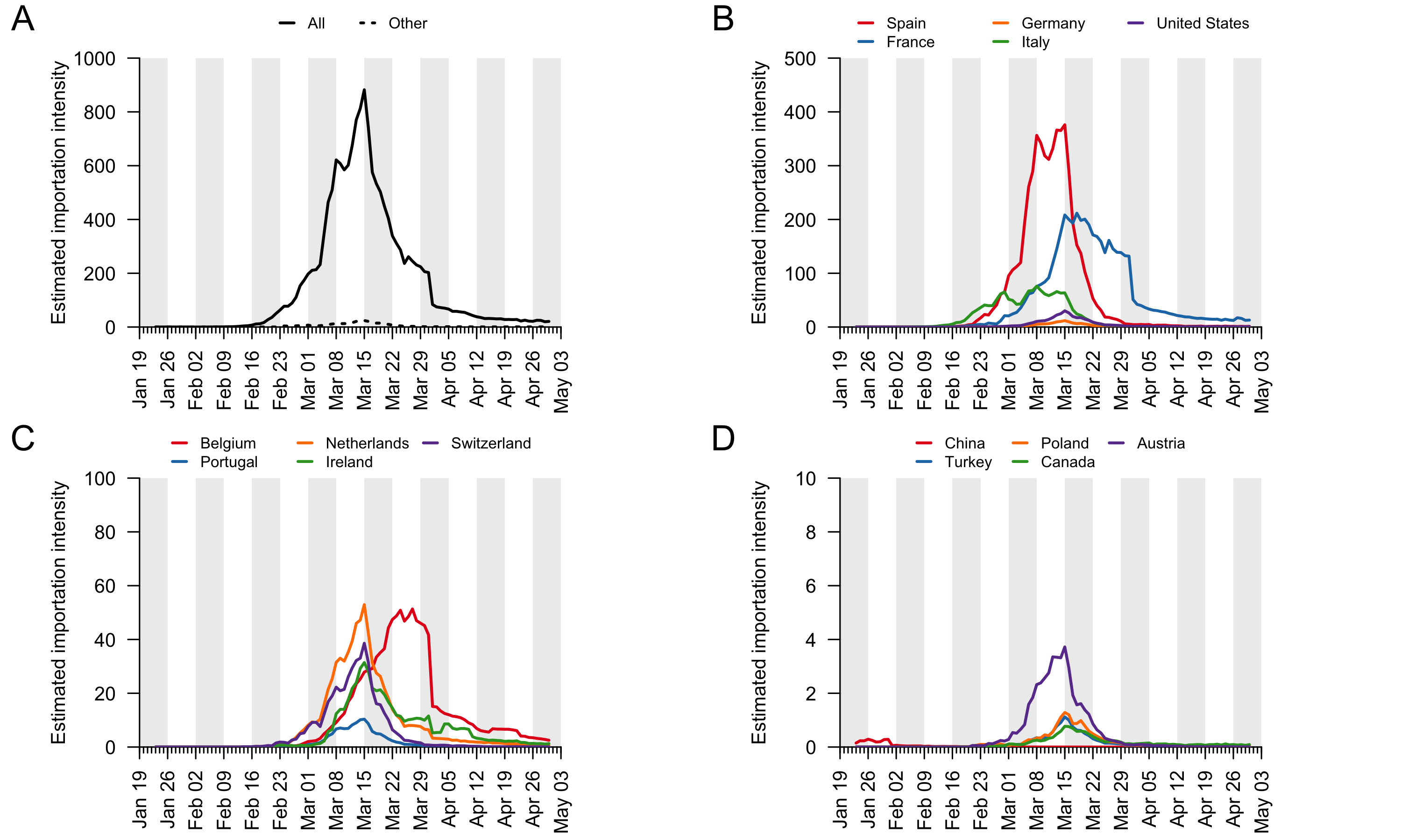
For each country, the estimated daily importation intensity (EII) is computed by multiplying the estimated proportion of people in each country who are infectious on each day (see item (ii) above) and the number of people entering the UK from that country on that day (see item (i) above). We estimated country-specific EII curves for all countries. We display the curves for those countries with the greatest net contribution to virus introduction (see Appendix 4). The EII curves for remaining countries were calculated and then aggregated into a single category “Other”. Here we use the EII as a measure of relative intensity through time and among countries. It is possible to interpret the global or country-specific EII values as the expected number of people entering the UK per day who are infectious. However, that interpretation requires us to assume that (i) the infection fatality rate used is accurate and constant across countries, and (ii) the probability of a traveller being infectious is the same as the proportion of the source country’s population that is infectious on the same day. We caution that further work is needed to evaluate whether these assumptions are reasonable.
No personal or individual-level information was used or analysed in this study.
Appendix
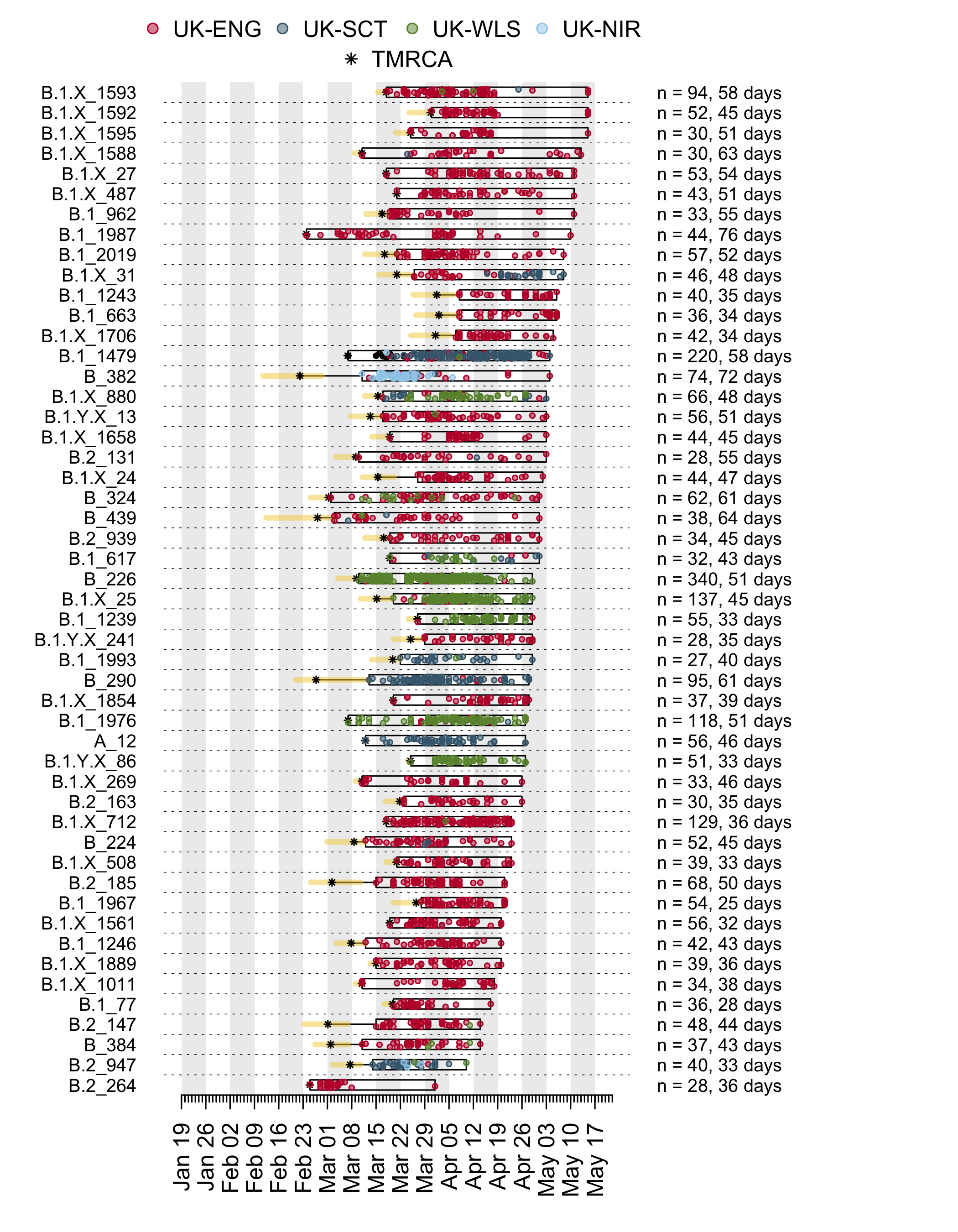
Appendix 1a: Illustration of the time course of the largest UK transmission lineages. Each row is a transmission lineage. Dots are genome sampling times (coloured by sampling location) and boxes show the range of sampling times for each transmission lineage. Asterisks show the median TMRCA of each lineage and the yellow bars show the 2.5% to 97.5% percentile range of each TMRCA. On the right, n indicates the number of genomes in the lineage, and the duration in days between the median TMRCA and most recently sampled genome is given.
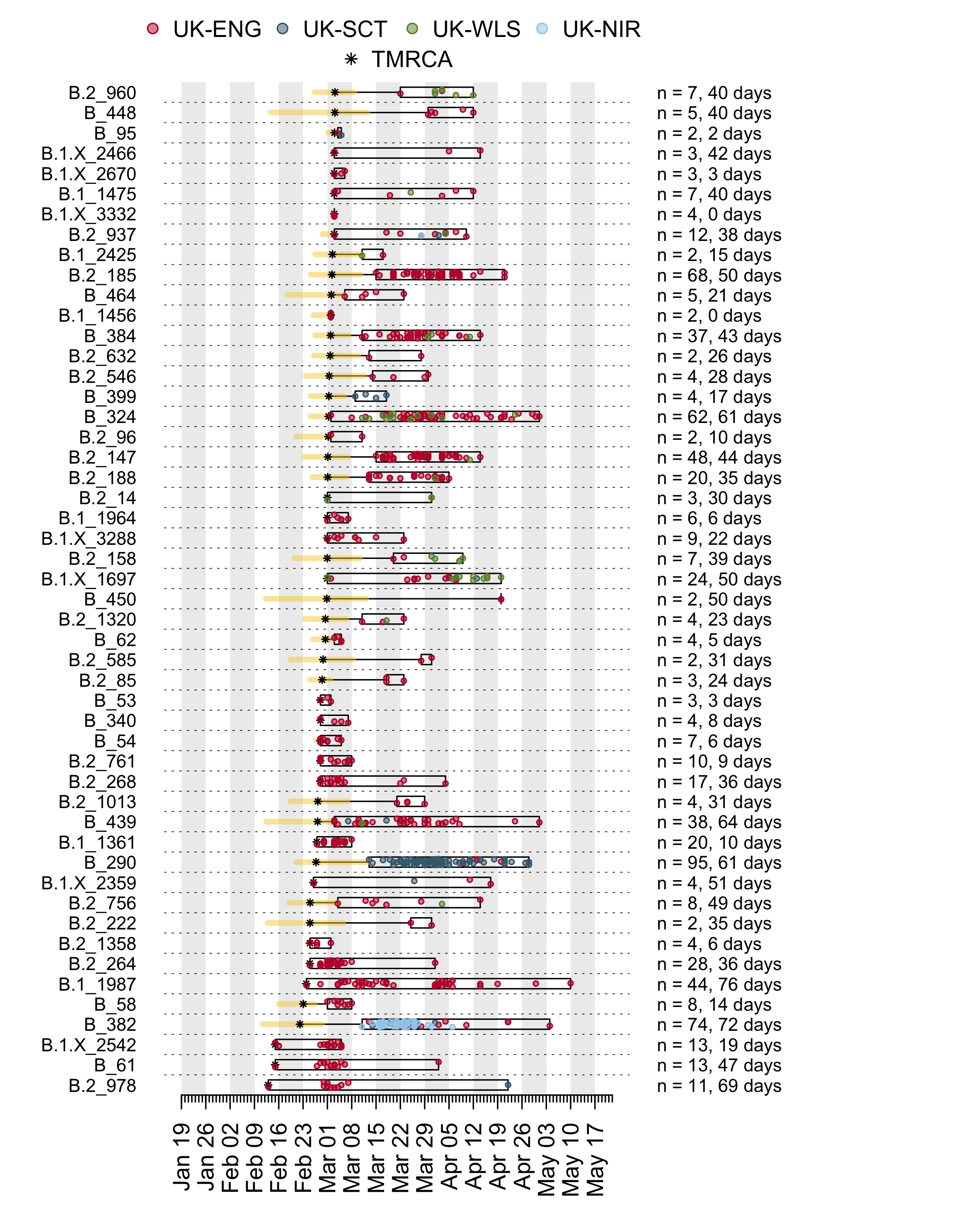
Appendix 1b: Illustration of the time course of the earliest UK transmission lineages. Each row is a transmission lineage. Dots are genome sampling times (coloured by sampling location) and boxes show the range of sampling times for each transmission lineage. Asterisks show the median TMRCA of each lineage and the yellow bars show the 2.5% to 97.5% percentile range of each TMRCA. On the right, n indicates the number of genomes in the lineage, and the duration in days between the median TMRCA and most recently sampled genome is given.
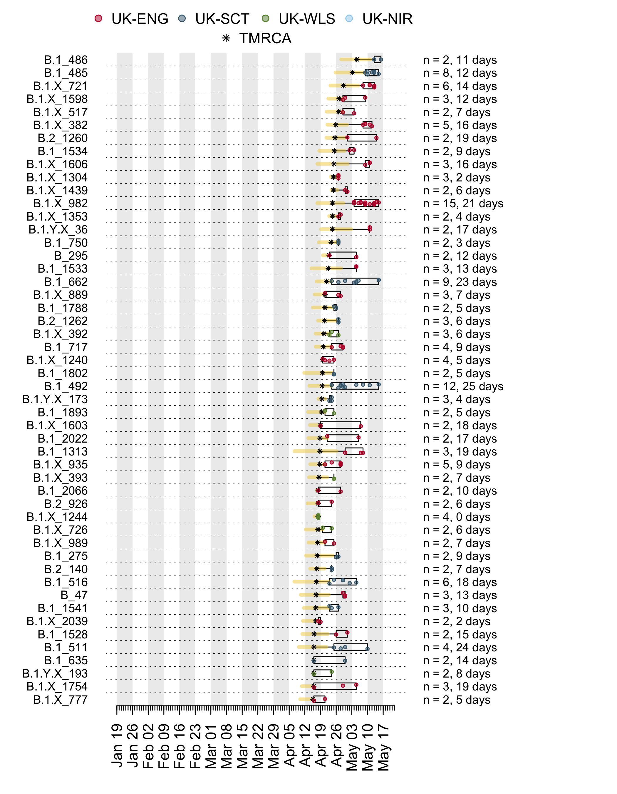
Appendix 1c: Illustration of the time course of the most recent UK transmission lineages. Each row is a transmission lineage. Dots are genome sampling times (coloured by sampling location) and boxes show the range of sampling times for each transmission lineage. Asterisks show the median TMRCA of each lineage and the yellow bars show the 2.5% to 97.5% percentile range of each TMRCA. On the right, n indicates the number of genomes in the lineage, and the duration in days between the median TMRCA and most recently sampled genome is given.
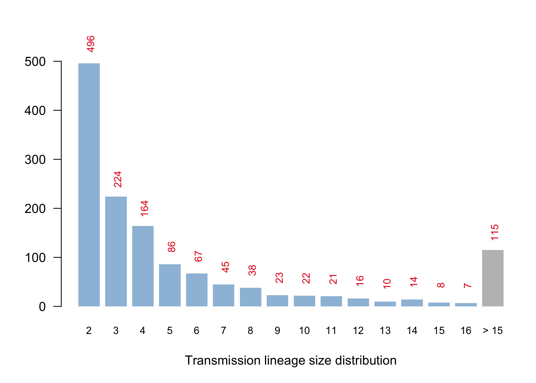
Appendix 2: Histogram of UK transmission lineage sizes (number of sampled virus genomes in each lineage). The number of lineages of each size is shown on the vertical axis and also in red text. In addition there were 6954 UK virus genomes that could not be reliably allocated to a transmission lineage due to either (i) limited virus genetic variation, or (ii) because only one genome had been sampled from the lineage. Many of these singletons will, in reality, belong to detected and undetected UK transmission lineages. The maximum number of detected transmission lineages that could be formed by these singletons is 3477. For related discussion see Footnote 4 in the main text.
Appendix 3: Estimated numbers of inbound travellers per day, and estimated number of active infections per day, for a range of countries (panels B-P). Panel A shows the total numbers for all countries combined (same as Figure 5).

Appendix 4: Estimated importation intensity (EII) curves for a range of countries with large COVID-19 epidemics or which experience high travel volumes with the UK (panels B-D). Panel A shows the EII for all countries (black line) and for all countries not in panels B-D (dotted line).