This was originally posted on http://epidemic.bio.ed.ac.uk/ebolavirus_evolutionary_rates
Over the summer 2014, Gire et al reported on an analysis of EBOV virus genomes sampled from 78 patients in May and June from Sierra Leone (along with 3 earlier genomes from March published by Baize et al.). This paper reported an estimate of the rate of evolution for the genome of approximately 2x10⁻³ substitutions per site per year. They also report an estimate for the rate of evolution of the Zaire EBOV lineage from 1976 to the present day of about 0.8x10⁻³ substitutions per site per year which is similar to estimates previously reported.
In March this year a further paper was published which contained additional 4 EBOV genomes sampled in Mali in September/October 2014 (Hoenen et al 2014). The rate they estimate is around 0.96x10⁻³ (i.e., similar to the long term rate estimate of EBOV and apparently lower than Gire et al.). An important point to note is that this new rate does not derive from the new data but from a reanalysis of the published Gire et al and Baize et al data (the rate they get with or without the Mali viruses is essentially the same). So why is there an apparent discrepancy between Gire et al.'s analysis and Hoenen et al.'s analysis of the same data? One obvious difference is that there is a different model being used. However, the result from Gire et al. is fairly robust to model choice (Figure 1). These estimates are slightly different from Gire et al in that they partition the data more to allow for variation in rate across different parts of the genome. Essentially the rate is high but the credible intervals are wide.
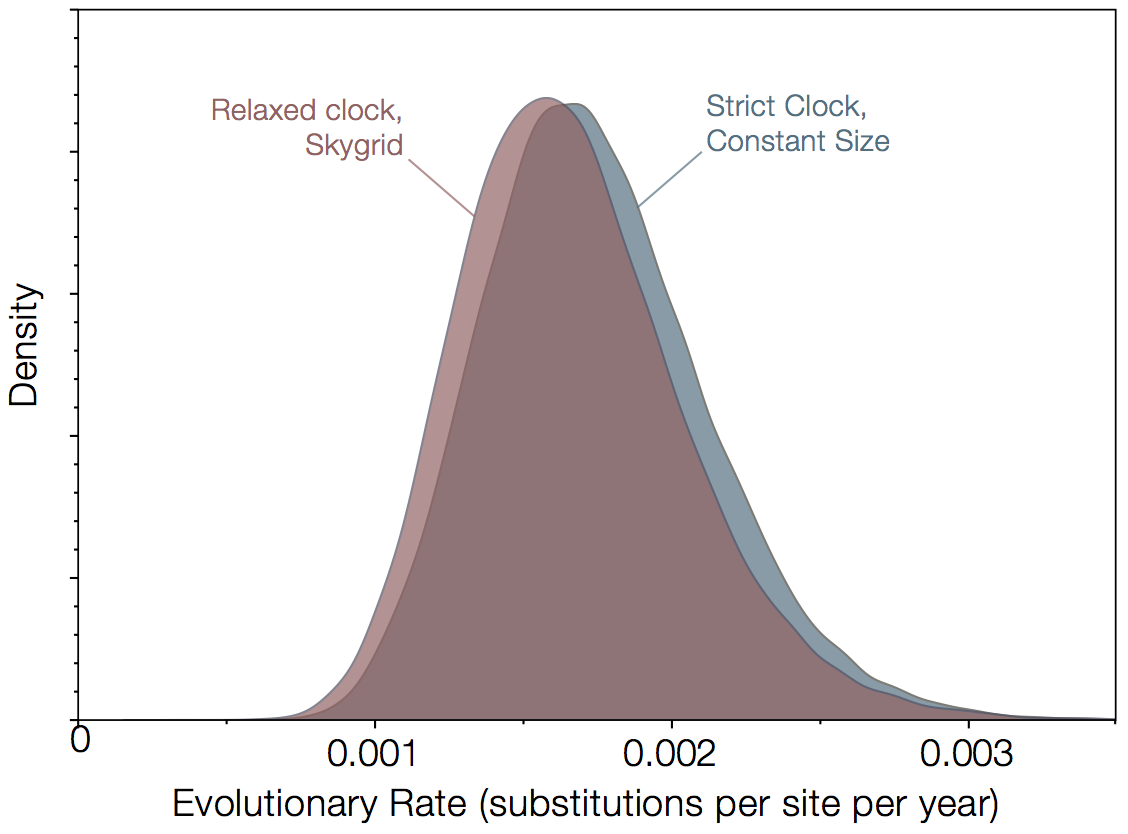
Figure 1|Rates of evolution estimated for 78 virus genomes from Gire et al (2014) and 3 from Baize et al (2014). Analysis was performed using BEAST for 2 extremes of evolutionary model - a strict molecular clock with a constant size population coalescent model against a relaxed molecular clock with the Skygrid non-parametric coalescent model.
A Bayes factor computed using a Stepping Stone Marginal Likelihood Estimate, finds that the relaxed clock + skygrid is preferred over the strict clock + constant size by a factor of about 20. We could dive deeper into which aspects of the model are important here but given the nearly identical rates estimated, this would be of limited interest.
Adding additional data
Gire et al. note the higher rate estimate and suggest this may be an observational artefact from seeing a short term excess of mildly deleterious variants that in the longer term would be eliminated from the population (purifying selection). The prediction here would be that as we observe viruses over a longer time period, the apparent rate would come down, not because the underlying rate is changing, but because these variants would comprise a deminishing proportion of the total observed changes. More generally, with a relatively limited span of sampling times (a few from March and the rest from a 6-week period in May/June) we expect more uncertainty in the rate over the short term.
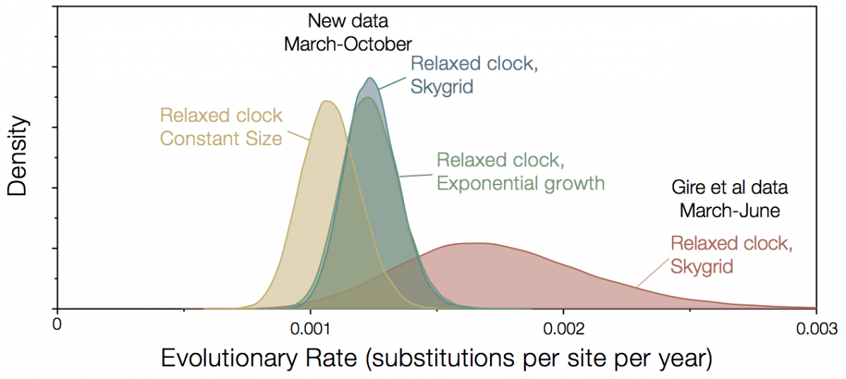
Since November last year, the Broad Institute, in partnership with Kenema Government Hospital and Tulane University have been releasing additional genomes from Sierra Leone. The full set now comprises 152 genomes sampled up until October 2015 and these are available for downloading here. This additional sampling period improves the estimates of rates considerably. The rate is now lower and has much narrower credible intervals (Figure 2). Choice of model is a little more important now, with constant size coalescent model giving a lower rate although exponential growth and Skygrid gave identical rates.
Figure 2|Rate estimates for Kenema/Broad data, left, compared with Gire et al data, right.
To decide which model provides the best fit we can estimate the marginal likelihood (MLE) using stepping-stone/path-sampling (Table 1). This scores each model for its goodness of fit to the data, taking into account the different complexities of the models. The model with the highest value is the best fit and the difference gives the log Bayes factor between the two.
Data	Clock	Tree	MLE
Gire	CLOC	CPC	-26704.05722
 	UCLN	SG	-26700.87374
New	CLOC	CPC	-29142.86777
 	CLOC	EGC	-29121.71729
 	CLOC	SG	-29101.88645
 	UCLN	CPC	-29127.17541
 	UCLN	EGC	-29107.74666
 	UCLN	SG	-29095.16915
Table 1|The marginal likelihood estimates for different models. Best fitting models are highlighted in bold. Generally UCLN relaxed clock models give a log Bayes factor of at least 7 over strict clock and the Skygrid gives a log Bayes factor of at least 12 over the next best coalescent model.
Random Notes
Marginal Likelihood estimates strongly support the UCLN relaxed clock and Skygrid over simpler models for both the Gire et al data and the newer set of 233.
In Gire et al (2014) we never claimed that Ebola virus was evolving faster in this outbreak but simply that the observed rate was high because the time frame was short. This is confirmed by the new data and the new rate estimate.
With this model, the newer data gives a rate of 1.24x10⁻³ substitutions per site per year with 95% CIs of 1.0x10⁻³, 1.45x10⁻³. I believe it is unlikely that further data will substantially change this estimate.
This estimate is still 1.5x higher than the long term, 1978-2014, between outbreak rate of 0.8x10⁻³ and does not include that value in its 95% CIs.
There is no reason to expect these rates to be the same. Most of the evolution in the long-term analysis has occurred in the animal reservoir even though the viruses themselves have been sampled from humans (albeit in much smaller outbreaks than the current one). Virus evolutionary rates can be different in different hosts due to a range of factors.
One final point is that knowing the rate of evolution tells us almost nothing about the likelihood of a virus to adapt to a host population.