Introduction
The phylogenetic analysis and visualization of SARS-CoV-2 genomic variation has played an important role in variant tracking, informing public health decisions, and scientific communication. However, the enormous number of SARS-CoV-2 genomes being contributed by laboratories around the world (with over one million genomes available at GISAID) present new challenges for phylogenetics.
Reconstructing trees by maximum likelihood is a time consuming and resource intensive process that does not readily scale to current amounts of SARS-CoV-2 data without aggressive down-sampling. We have been developing a new open source framework (GitHub - PoonLab/covizu: Rapid analysis and visualization of coronavirus genome variation, MIT license) for processing and visualizing SARS-CoV-2 genome diversity in near “real time”. This resource was initially brought online in May 2020 and became provisioned by GISAID at CoVizu in December 2020.
In brief, we extract genetic differences from the SARS-CoV-2 reference genome as a feature vector for each genome, and use non-parametric bootstrapping and neighbor-joining tree reconstruction to generate a consensus tree relating samples within each PANGO lineage. Each lineage-specific tree is rendered as an interactive beadplot in which samples with effectively identical genome sequences are collected into variants. These objects are serialized and rendered as interactive support vector graphics using the D3js JavaScript framework.
Usage
The CoVizu web resource consists of a single page, partitioned into three major panels.
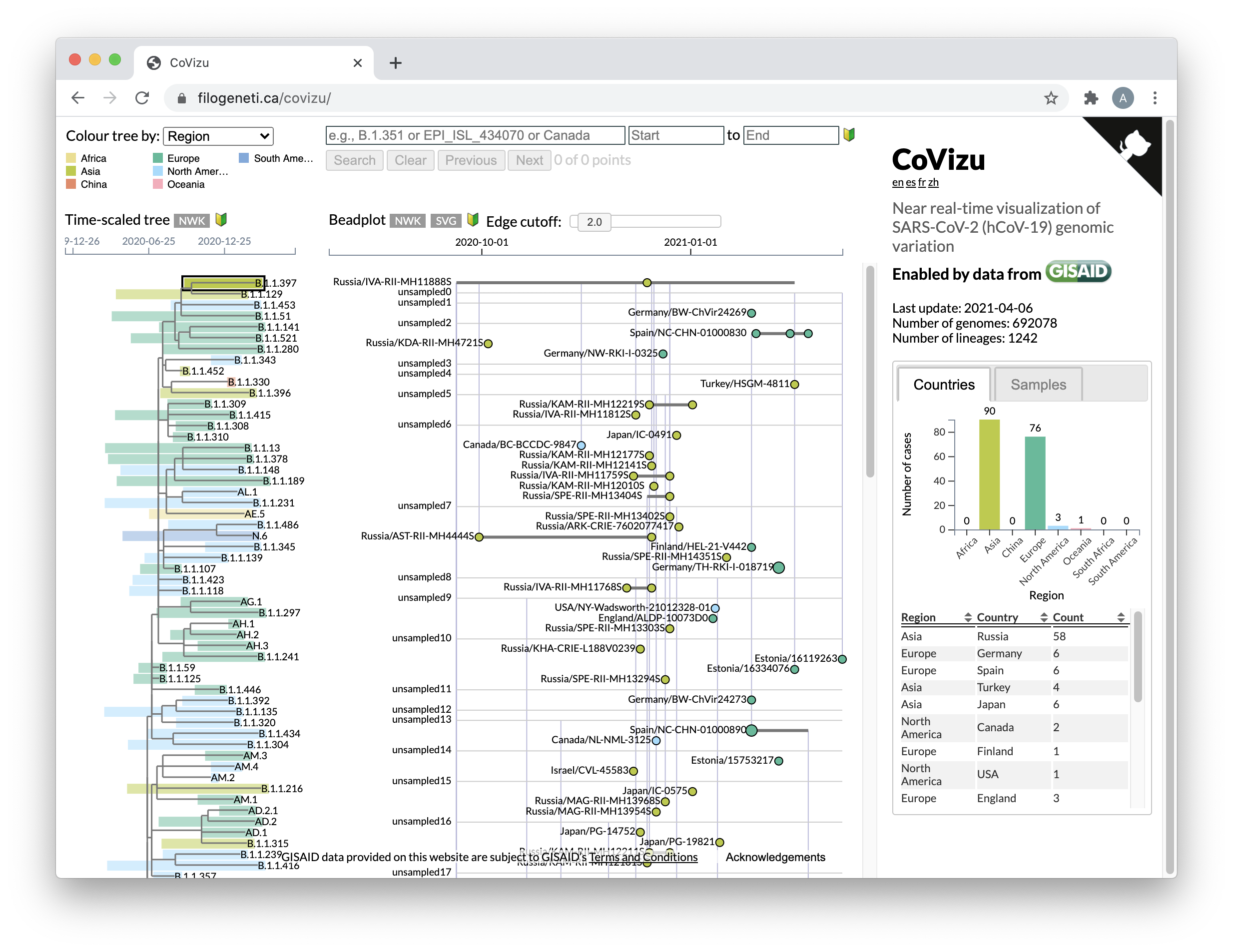
Figure 1 | Overview of CoVizu web page layout.
A time-scaled tree relating PANGO lineages is rendered on the left panel. Each tip representing a lineage is labelled with the lineage name, and annotated with a coloured rectangle that corresponds to the range of sample collection dates. By default, rectangles are coloured by the most common geographic region of samples for that lineage. Users may also colour lineages by number of samples, most recent collection date, and divergence from the molecular clock. Tooltips associated with each rectangle provide summaries of common lineage mutations and its distribution among countries.
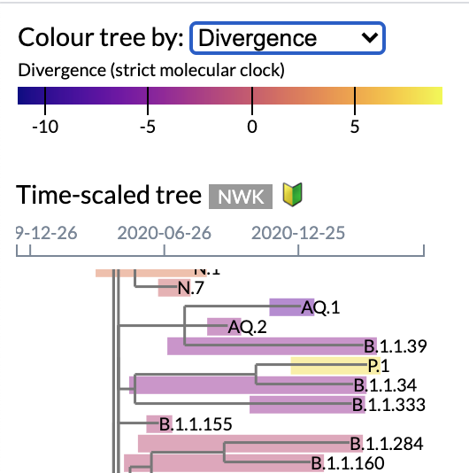
Figure 2 | Focus on time-scaled tree interface, featuring lineage colouring by divergence from molecular clock.
Clicking on a lineage displays the associated “beadplot” in the middle panel. Samples with identical genome sequences (“variants”) are represented by circles on a horizontal line, where their positions correspond to sample collection dates. The area of each circle is proportional to the number of samples with the same collection date, and colours correspond to the most common geographical region.
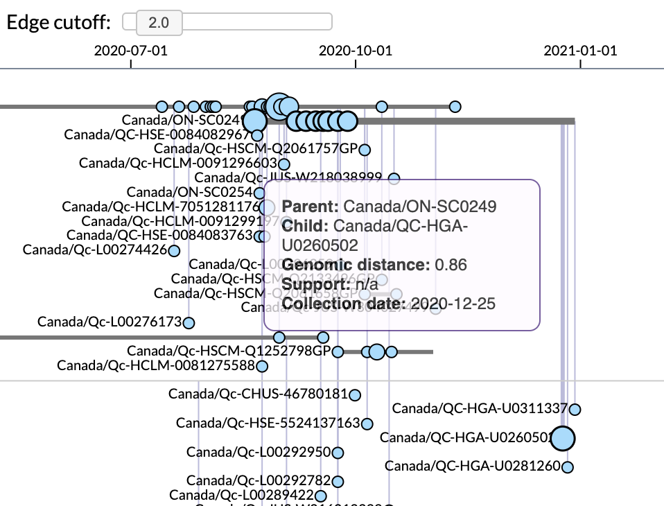
Figure 3 | Focus on beadplot visualization of samples within a lineage, featuring tooltip details associated with a vertical edge.
Variants are connected by vertical edges that represent branches in the consensus neighbor-joining tree. Branches with low bootstrap support or mean length below 0.5 genetic differences are collapsed, such that tip labels can be reassigned to internal nodes. Thin grey lines represent unsampled ancestral variants that do not carry any tip labels. A slider widget can be used to filter edges by branch lengths.
The right-most panel displays two tabbed sub-panels. A “Countries” sub-panel displays a barplot of sample frequencies by geographic region, and a table (with sortable columns) that displays a breakdown of samples by country. Both are updated in response to user selections in the time-tree and beadplot panels. The “Samples” sub-panel displays a table of all samples in the selected lineage, variant, or “bead”. Hovering over an accession number displays the originating and submitting lab and author information associated with that sample.
A search interface is provided at the top of the page. The text input field recognizes and autocompletes PANGO lineage names and GISAID accession numbers. In addition, users may input any substring for an exact search of all samples, and limit the search to a range of collection dates.
Methods
The back-end pipeline is currently run on even numbered days. Data provisioned by GISAID are downloaded and processed in Python. Records are excluded if they lack PANGO lineage assignments, represent non-human samples, have sequences less than 29,000 nt in length, or have incomplete dates of sample collection. Next, we stream the filtered genome sequences to minimap2 for pairwise alignment against the reference genome (NC_045512).
The minimap2 SAM output stream is redirected into Python and parsed to extract all genetic differences (including insertions and deletions) from the reference as features. At this stage, we filter known problematic sites and genomes with more than 300 uncalled bases. We also exclude genomes that are under- or over-divergent from the molecular clock expectation given their collection dates, assuming a Poisson distribution around a mean of 0.0655 substitutions/genome/day (Rambaut et al, 2020) and an origin date of 2019-12-01.
For each lineage, we select the most recent genome passing these filters as the representative sample, generate a multiple sequence alignment by excluding all insertions relative to the reference genome, and use FastTree to reconstruct a maximum likelihood tree relating lineages. Next, we use TreeTime to rescale this tree in time under a fixed molecular clock (0.0655/genome/day). The resulting Newick tree string is deserialized client-side into a rectangular layout augmented with lineage-specific data using the D3.js framework.
For each lineage, we merge genomes with identical feature vectors into a single “variant”. We compute the symmetric differences between feature vectors every pair of variants. Next, we randomly resample the feature set union (i.e., all features observed in any genome) 100 times with replacement, and then apply the results to reweigh the original symmetric differences to yield 100 pairwise distance matrices. We use each matrix as input for neighbor-joining tree reconstruction with RapidNJ, and generate a consensus tree from the outputs. All branches with a mean length below 0.5 or bootstrap support below 50% are collapsed, transferring any tip labels to the ancestral node. Finally, we serialize the resulting beadplot data into a JSON object.
Contributors
CoVizu was developed by Roux-Cil Ferreira, Emmanuel Wong, Kaitlyn Wade, Molly Liu, Laura Muñoz Baena, Gopi Gugan, Abayomi S. Olabode and Art F. Y. Poon, at the Department of Pathology and Laboratory Medicine, Western University, Canada.
References
Li H. Minimap2: pairwise alignment for nucleotide sequences. Bioinformatics. 2018 Sep 15;34(18):3094-100.
Price MN, Dehal PS, Arkin AP. FastTree 2–approximately maximum-likelihood trees for large alignments. PLoS ONE. 2010 Mar 10;5(3):e9490.
Rambaut A, et al. Phylodynamic Analysis — 176 genomes — 6 Mar 2020. Phylodynamic Analysis | 176 genomes | 6 Mar 2020 ; accessed 2020-11-24.
Sagulenko P, Puller V, Neher RA. TreeTime: Maximum-likelihood phylodynamic analysis. Virus Evolution. 2018 Jan;4(1):vex042.
Simonsen M, Mailund T, Pedersen CN. Inference of large phylogenies using neighbour-joining. In International Joint Conference on Biomedical Engineering Systems and Technologies 2010 Jan 20 (pp. 334-344). Springer, Berlin, Heidelberg.
Turakhia Y, De Maio N, Thornlow B, Gozashti L, Lanfear R, Walker CR, Hinrichs AS, Fernandes JD, Borges R, Slodkowicz G, Weilguny L. Stability of SARS-CoV-2 phylogenies. PLoS Genetics. 2020 Nov 18;16(11):e1009175.