Phylodynamic analyses based on 128 sequences
Jérémie Sciré1,2, Timothy G. Vaughan1,2, Sarah A. Nadeau1,2, and Tanja Stadler1,2,*
1Department of Biosystems Science and Engineering, ETH Zürich, Basel, Switzerland
2Swiss Institute of Bioinformatics (SIB), Switzerland
*Correspondence to be addressed to: [email protected]
March 6th 2020
In this report, we outline phylodynamic analyses based on full-length SARS-CoV-2 genomes downloaded from GISAID. Acknowledgements for and details of the genome sequences are given in Table 3.
The “full alignment” of 128 sequences was obtained following the exact same procedure as described in the post by A. Rambaut. We considered a second alignment, coined the “cluster-free alignment”, where only one representative from each known epidemiologically-linked transmission cluster was included (obtained as in post), resulting in a 86-sequence alignment. The third considered alignment is the “outside-China alignment” where we eliminated all sequences sampled within China from the cluster-free alignment, resulting in 41 sequences.
We use these three alignments in BEAST2 [1] in order to quantify:
- Clock rate (i.e. an evolutionary dynamics aspect)
- TMRCA and time of origin of the outbreak (TMRCA = time of most recent common ancestor of the samples; this is a proxy for the time of origin of the outbreak, i.e. an important past state of the epidemic)
- R0 and Re (i.e. an epidemiological dynamics aspect)
- Overall number of cases (i.e. an important current state of the epidemic)
Evolutionary analysis: Quantifying clock rate and TMRCA
The product of clock rate and TMRCA can generally be inferred from genetic sequencing data. However, the clock rate and the TMRCA are non-identifiable in the absence of measurable evolution; we also call this the absence of clock signal. Several posts explored the amount of clock signal in the COVID-19 sequencing data (A. Rambaut, S. Duchene, L. du Plessis, O. Pybus & L. du Plessis). We explored the sensitivity of the clock rate estimates to the choice of tree prior, similar to what was done for the early sequences in the 2013 - 2016 Ebola outbreak [3].
Method
We chose a number of coalescent and birth-death based tree priors and inferred the phylogenetic trees together with the evolutionary and epidemiological parameters. The choice of models and prior distributions for the model parameters is shown in Table 1.
In summary, we have three different coalescent frameworks and three different birth-death frameworks. For the birth-death framework, we additionally have three different options for the priors on the removal rate δ. In total, we thus perform twelve analyses both on the full alignment and on the cluster-free alignment. The rational for considering the cluster-free alignment is that epidemiologically-linked transmission clusters have been mentioned to potentially bias clock rate estimates, see discussion below this post.
For the structured models, we assigned each tip one of three demes at random. For birth-death models, we further analytically integrate over the tip deme assignment as explained in [6]. Such deme assignment is envisioned to take into account population structure implicitly.
For each analysis, we run five parallel chains for 1×10⁸ to 2.5×10⁸ steps, depending on the tree prior configuration. We check the convergence of each individual chain (ESS > 200) and combine them to obtain the final posterior distribution. Structured coalescent runs mixed more slowly, in this case, we set the threshold for convergence to ESS > 100 for individual chains.
| Model | Parameter | Prior distribution |
|---|---|---|
| Strict clock | clock rate | lognormal(-7, 1.75) |
| HKY | kappa | lognormal(1.0, 1.25) |
| Gamma shape | Exponential(0.5) | |
| Coalescent | Ne | lognormal(1, 2); lognormal(1, 1.5) (with structure) |
| exponentially growing population | growth rate r | laplace(0, 20) |
| with structure [4] | migration rate | lognormal(1, 1.5) |
| Birth-death [7] | Re | lognormal(0.8, 0.5) |
| removal rate δ | lognormal(3, 0.8); fixed to 365/10 per year; fixed to 365/20 per year | |
| sampling proportion s | beta(alpha = 1, beta = 50) | |
| time of origin tor | lognormal(-1.5, 0.4) | |
| skyline [7] | change time for Re, s | fixed to Jan. 23 (start of Wuhan quarantine) |
| with structure [2, 5] | migration rate | lognormal(1, 1.5) |
Table 1: Models and prior distributions used for the BEAST2 analyses. If no reference is provided for a model, this model is part of the core of BEAST2 [1]. We highlight that 1/δ is the time of an individual being infected, i.e. the sum of the exposed period and the infectious period. We both estimate δ, or assume 1/δ to be fixed to 10 or 20 days. Sampling is assumed to coincide with removal from the infectious pool. Under the birth-death skyline model, the parameters Re and s are allowed to change.
Results
The resulting estimates for clock rate, TMRCA, tree length (i.e. sum of branch lengths), and tree divergence (= clock rate x tree length) are shown in Figure 1. As expected, the tree divergence is estimated the same across tree prior choices. The clock rate estimate and the tree height (resp. tree length) estimate are inversely correlated. The clock rate estimates for the full alignment are higher compared to the cluster-free alignment. Since the priors do not take into account the epidemiologically-linked transmission clusters, we focus now on the cluster-free alignment results.
The clock rate estimates for the unstructured coalescent are around 0.8x10⁻³ (median) while all birth-death estimates with a fixed δ and the structured coalescent estimates are lower, with the smallest median estimates being a bit under 5×10⁻⁴. The unstructured coalescent estimates agree with previous estimates (all based on the unstructured coalescent; Table 2). Across all the analyses we ran, the median TMRCA was estimated to be between early November and mid-December 2019.
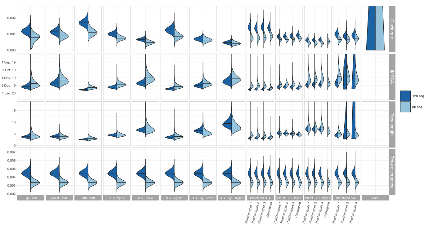
Figure 1: Posterior distribution of clock rate, TMRCA, tree length (i.e. sum of branch lengths), and tree divergence (= clock rate x tree length) for the 12 different tree prior choices. The tree length is in units of years and the clock rate is in units of substitutions / site / year.
| Median | HPD low | HPD high | Author |
|---|---|---|---|
| 0.80 × 10⁻³ | 0.14 × 10⁻³ | 1.31 × 10⁻³ | A. Rambaut (24/02) |
| 0.92 × 10⁻³ | 0.33 × 10⁻³ | 1.46 × 10⁻³ | A. Rambaut (12/02) |
| 1.23 × 10⁻³ | 5.63 × 10⁻⁴ | 1.98 × 10⁻³ | S. Duchene (03/02) |
| 1.05 × 10⁻³ | 3.29 × 10⁻⁴ | 2.03 × 10⁻³ | K. Andersen (27/01) |
Table 2: Previous clock rate estimates for SARS-CoV-2 based on the unstructured coalescent tree prior.
| Model | tMRCA | clock rate |
|---|---|---|
| birth-death model, strict clock | 27.11.2019 [07.11.2019; 11.12.2019] | 7.4 x 10⁻⁴ [4.9 x 10⁻⁴; 1.02 x 10⁻³] |
| structured birth-death model, strict clock | 28.11.2019 [08.11.2019; 14.12.2019] | 6.7 x 10⁻⁴ [4.5 x 10⁻⁴; 9.2 x 10⁻⁴] |
Table 3: We provide the numerical values for two representative analyses of the cluster-free alignment shown in Figure 1 (namely column 4 and 11). These two birth-death models assume the duration of infection until being non-infectious (=1/δ) to be 10 days.
Epidemiological analysis: R0, Re, the time of origin of the epidemic, and the overall number of cases
Next we set out to quantify the epidemiological dynamics. We should be close to the phylodynamic threshold such that these analyses reveal informative insights into epidemic spread, see a post by E. Volz. T. Bedford reported prevalence and incidence estimates based on the genomic data. Here, we estimate R0, Re, the time of origin of the epidemic, the total number of cases, and the sampling proportion using birth-death models.
Method
We apply the birth-death skyline framework to the cluster-free alignment and the outside-China alignment, with both Re and s being allowed to change through time. The full alignment is not considered here as the sampling assumption of the birth-death model is strongly violated in the presence of the epidemiologically-linked transmission clusters.
In addition to the cluster-free alignment, we analysed the outside-China alignment as sampling intensity within China and outside of China is very different. Further, we are not confident to assume uniformly-at-random sampling (specified by the parameter s) within China. We argue that the outside-China sequences can be viewed as a very sparse and random sample from the pool of Chinese sequences. In particular, a case is sampled and sequenced if an infected individual travels abroad and they (or a closely linked epidemiological case) is subsequently diagnosed and sequenced. The sampling proportion s is thus a combination of travel abroad, diagnosis, and sequencing. As travel abroad changed drastically upon the start of the Wuhan quarantine, we allow s to change at that time point. We also added a third time interval (after Feb. 1st) to account for the reduced amount of available samples after that date in this dataset.
Here we assume a prior for the sampling proportion s different from what is shown in Table 1; namely, we assume uniform priors for the sampling proportion. The lower bound is 0 for both alignments and the three time intervals. The upper bounds for the three intervals, in time order from past to present, are 0.1, 0.0025, and 0.00025 for the cluster-free alignment and 0.02, 0.0025, and 0.0002 for the outside-China alignment. The upper bounds for these uniform priors were determined based on the number of sequences and the number of confirmed cases (WHO situation reports).
We argue that the duration of an infection (parameter δ) did not drastically change throughout this epidemic outbreak and in particular fixed it to two plausible values, 365/10 and 365/20 per year, as above. As the clock rate estimate is uncertain (see above), we fixed the clock rate here to two different plausible values, namely 10−3 and 5 × 10⁻⁴.
The other priors were set as in Table 1. Chain length and convergence assessment was done as for the evolutionary analyses.
Results
The parameter estimates are shown in Figure 2. For China, the median Re before Jan. 23 (which we refer to as R0) is estimated to be between 2.5 - 7.5 based on the outside-China sequences; R0 is estimated to be lower based on the cluster-free sequences.
The median of the total number of cases (= # sequences / sampling proportion) is estimated to be around 1’000 - 10’000 at the time of the Wuhan quarantine (Jan. 23, 2020). The confirmed number of cases on that day is 581 with 571 being from China (WHO situation reports). We do not trust the estimates after the start of the quarantine, see caveats below.
The TMRCA is a bit younger than the time of origin of the outbreak, the estimated medians differ by around 1 week.
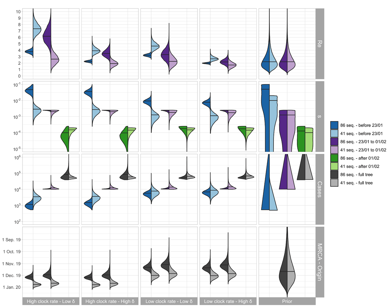
Figure 2: Posterior distribution of Re before Wuhan quarantine (which can be interpreted as the R0), Re after Wuhan quarantine, sampling proportion s, total number of cases (= # sequences / s), time of origin, and TMRCA for the cluster-free and the outside-China alignment. In the bottom row, in each panel, we show on the left the estimated TMRCA and on the right the estimated time of origin of the epidemic.
We argue that the outside-China alignment fulfills our model assumptions regarding the sampling better than the cluster-free alignment. Second, based on recent results, we argue that a δ = 365/10 is reasonable. Third, we argue that structured models more accurately quantify the clock rate compared to unstructured models [3] and thus are most confident in the results with the clock rate of 5x10⁻⁴ (see results in Figure 1). We include sequences collected after Jan. 23 in our analysis because the sampled transmission events leading to these sequences may have occurred prior to the 23rd, i.e. during our time interval of interest. However, we do not trust the epidemiological estimates after Jan. 23 since the epidemic became highly structured after this point. For example, Wuhan was under quarantine beginning that day. In summary, we are most confident in the estimates shown in light blue in Figure 2 in the “Low clock rate – High δ” column. In the following summary section, we highlight these results.
Summary
Overall, the clock rate and tree height estimates are sensitive to the prior, with the clock rate medians varying by about a factor of 2 and the tree height medians by about 1 month. Additional sequences should make these estimates more robust towards the tree prior choice.
For what we argue are the most reasonable model assumptions based on today’s knowledge, the R0 for the Chinese epidemic is estimated to be between 2 - 3.5. The number of total cases is estimated to be between 2’000 - 30’000 at the time of the Wuhan quarantine (although only 571 cases were confirmed). Thus the underreporting appears very severe, with only 1 in 3.5 to 1 in 50 cases being reported. The start of the epidemic is estimated to be between mid-October and mid-November. The most recent common ancestor giving rise to the outside-China sequences is estimate to be about 3 weeks later.
Caveats
A more in-depth discussion of the caveats regarding the evolutionary analysis is available in previous posts (A. Rambaut, S. Duchene, L. du Plessis); the same caveats apply here.
For the epidemiological analysis, the non-random mixing of the epidemic (particularly after the beginning of the Wuhan quarantine) and the non-constant sampling effort are potential strong sources of bias in the estimates.
Acknowledegments
We thank Andrew Rambaut for his help and guidance with the processing of the GISAID sequences. We gratefully acknowledge the Authors and the Originating and Submitting Laboratories for their sequence and metadata shared through GISAID, on which this research is based. Below is a full table containing the sequences used for the analysis.
Table 4: SARS-CoV-2 genome sequences used in this analysis, the GISAID accession numbers, and submitting labs.
References
-
Remco Bouckaert, Timothy G. Vaughan, Joelle Barido-Sottani, Sebastián Duchêne, Mathieu Fourment, Alexandra Gavryushkina, Joseph Heled, Graham Jones, Denise Kühnert, Nicola De Maio, et al. Beast 2.5: An advanced software platform for bayesian evolutionary analysis. PLoS computational biology, 15(4):e1006650, 2019.
-
Denise Kühnert, Tanja Stadler, Timothy G. Vaughan, and Alexei J. Drummond. Phylodynamics with migration: a computational framework to quantify population structure from genomic data. Molecular biology and evolution, 33(8):2102–2116, 2016.
-
Simon Möller, Louis du Plessis, and Tanja Stadler. Impact of the tree prior on estimating clock rates during epidemic outbreaks. Proceedings of the National Academy of Sciences, 115(16):4200–4205, 2018.
-
Nicola F. Müller, David Rasmussen, and Tanja Stadler. Mascot: parameter and state inference under the marginal structured coalescent approximation. Bioinformatics, 34(22):3843–3848, 2018.
-
Jérémie Sciré, Jöelle Barido-Sottani, Denise Kühnert, Timothy G. Vaughan, and Tanja Stadler. Improved multi-type birth-death phylodynamic inference in beast 2. bioRxiv, 2020.
-
Tanja Stadler and Sebastian Bonhoeffer. Uncovering epidemiological dynamics in heterogeneous host populations using phylogenetic methods. Philosophical Transactions of the Royal Society B: Biological Sciences, 368(1614):20120198, 2013.
-
Tanja Stadler, Denise Kühnert, Sebastian Bonhoeffer, and Alexei J. Drummond. Birth–death skyline plot reveals temporal changes of epidemic spread in HIV and hepatitis C virus (HCV). Proceedings of the National Academy of Sciences, 110(1):228–233, 2013.
Summary
This text will be hidden