Phylogenetic analysis of nCoV-2019 genomes
6-Mar-2020
Andrew Rambaut, University of Edinburgh, Edinburgh UK
[email protected]
This is a brief report outlining a simple phylogenetic analysis of publicly shared genome sequences. It gives some preliminary findings for information purposes is not intended as an academic work. All the data used here is provided by the laboratories listed below through NCBI or GISAID.
Phylogenetic analysis
This analyses uses 176 full-length genomes kindly made available on the GISAID and NCBI Genbank platforms. Some sequences were omitted as they were too short, contain sequencing artefacts, were resequencing of the same sample or had insufficient associated information. By ‘sequencing artefacts’ I mean apparent nucleotide variation that is probably due to the process of sequencing or bioinformatics pipelines - most likely due to the difficulty of sequencing samples with low concentrations of virus. Removing these sequences (or in some cases masking out the artefacts) is to avoid potential biases these may cause.
Acknowledgements and details of the genome sequences used in this analysis are given in Table 6 at the end of this document.
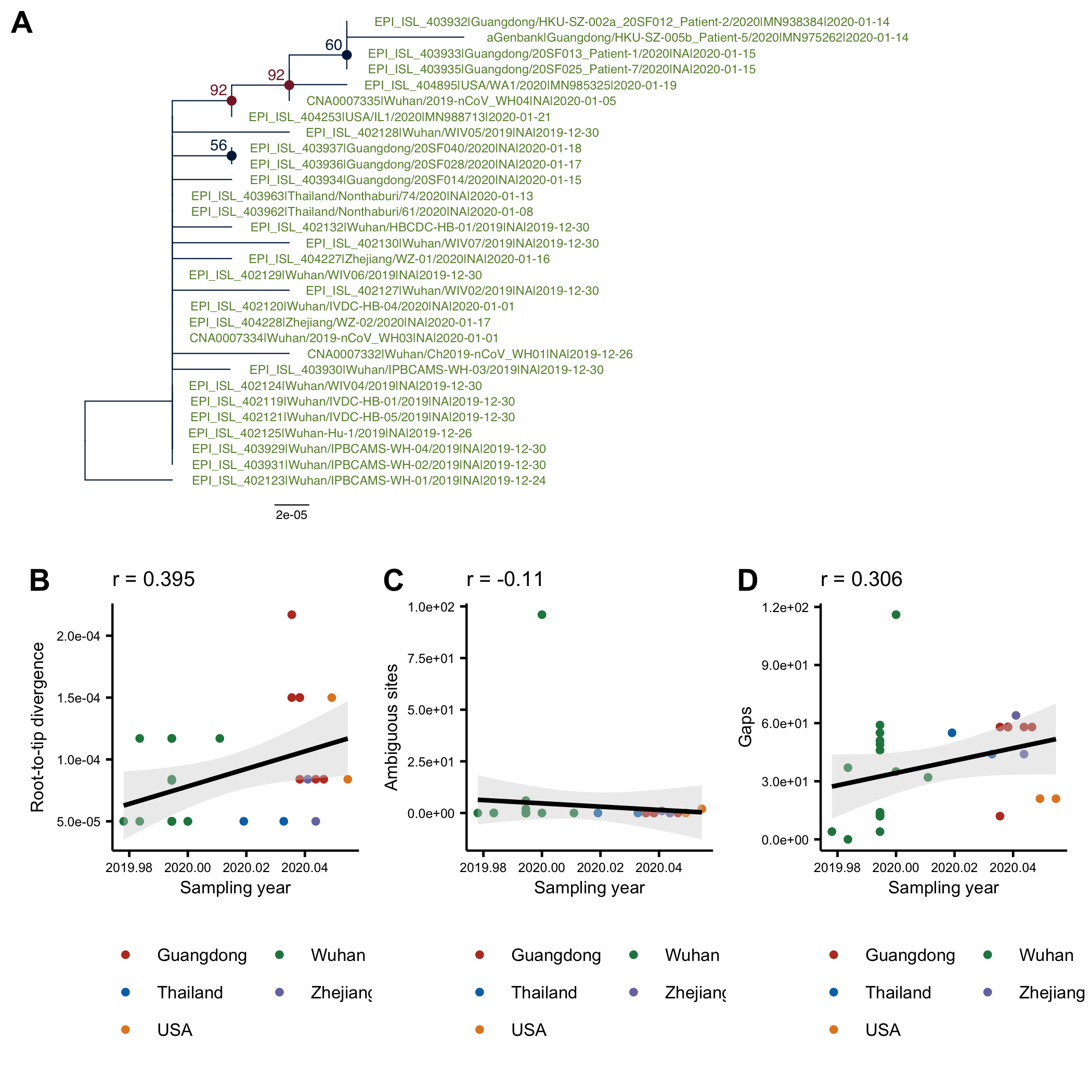
The phylogenetic tree of the currently available complete genomes is given in Figure 1. This shows that there is limited genetic variation in the currently sampled viruses but more recent ones are showing more divergence as is expected for fast evolving RNA viruses. But the lack of diversity is indicative of a relatively recent common ancestor for all these viruses.
Figure 1 | Maximum likelihood tree of nCoV2019 genomes constructed using PhyML [1]. The tree is rooted using the oldest sequence but this is an arbitrary choice. Interactive tree figure by @john.mccrone using figtree.js.
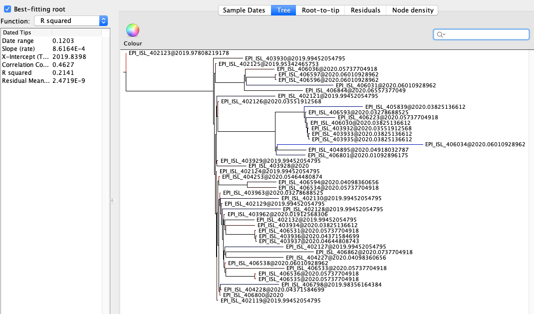
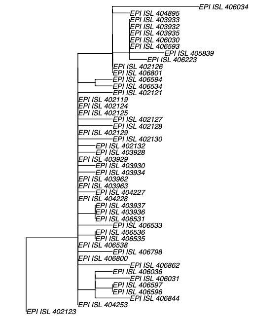
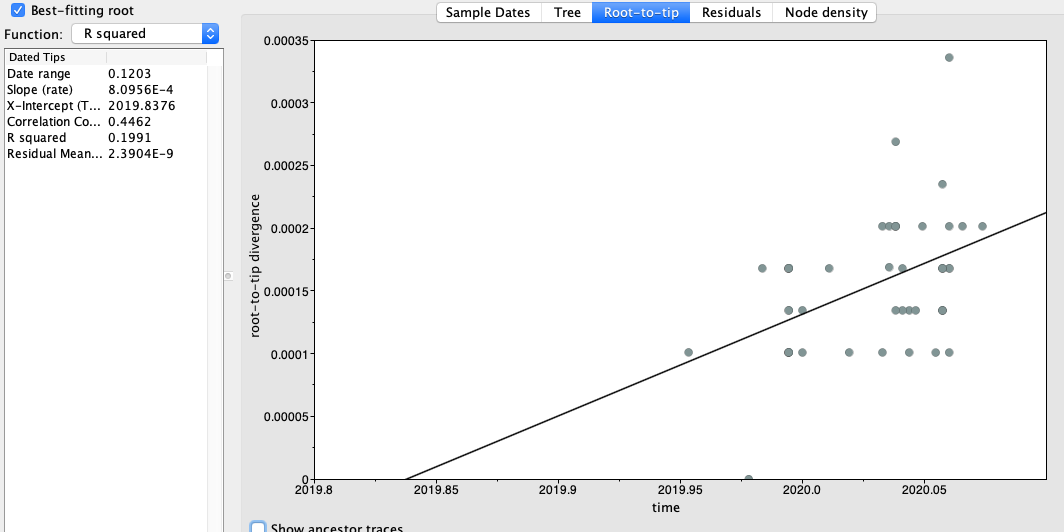
Figure 2 | Maximum likelihood tree of nCoV2019 genomes constructed using PhyML [1] and a root-to-tip divergence plot. Click on branches to re-root the tree. Interactive tree figure by @john.mccrone using figtree.js.
Estimating the date of origin
The software package BEAST [2,3] was used to estimate the date of the most recent common ancestor (MRCA) of the currently available genomes. The MRCA represents the point where the ancestral virus of all the sampled cases was in the same host (whether this was a non-human animal or a human). The rate of evolution of the virus is estimated from the data.
A coalescent model is used as the prior on the tree with two different variants being used - the constant size and exponential growth models. Because the coalescent model assumes that we have a small random sample from a large population, only a single representative genome of any known epidemiologically-linked transmission clusters was included. This leaves 86 genomes in the analysis.
| Data | Coalescent model | Estimated rate | 95% interval |
|---|---|---|---|
| 12-Feb, 75 genomes | Exponential growth | 0.92x10⁻³ | 0.33x10⁻³ – 1.46x10⁻³ |
| 24-Feb, 86 genomes | Exponential growth | 0.80x10⁻³ | 0.14x10⁻³ – 1.31x10⁻³ |
Table 1 | The estimated rate of evolution (substitutions per site per year) of the sampled nCoV-2019 genomes. Note that recent data strongly supports a model of growth so in the interest of brevity I am no longer reporting the constant size model.
| Data | Coalescent model | Estimated TMRCA | 95% interval |
|---|---|---|---|
| 12-Feb, 75 genomes | Exponential growth | 29-Nov-2019 | 28-Oct-2019 – 20-Dec-2019 |
| 24-Feb, 86 genomes | Exponential growth | 17-Nov-2019 | 27-Aug-2019 – 19-Dec-2019 |
Table 2 | The estimated date of the MRCA of the sampled nCoV-2019 genomes.
The estimated dates for the most recent common ancestor (and the 95% credible interval) are compatible with the TMRCA from the beginning to middle of December (Table 2). The earliest reported date of symptom onset for the initial cluster of pneumonia cases was 1st December 2019 [4].
Exponential Growth
The exponential growth coalescent model can also infer a growth rate from the genome data, independent of any epidemiological information and from this calculate the doubling time (Table 3).
| Data | growth rate (/year) | 95% interval | doubling time (days) | 95% interval |
|---|---|---|---|---|
| 12-Feb, 75 genomes | 41.03 | 20.56 – 62.17 | 6.2 | 4.1 – 12.3 |
| 24-Feb, 86 genomes | 35.38 | 15.49 – 53.47 | 7.2 | 4.7 – 16.3 |
Table 3 | The estimated growth rate and doubling time.
Interpretation
Most estimates since the first data was produced have produced a date that is consistent with the epidemiological reports of a first cluster of cases in December at a seafood market in Wuhan City. As more genomes have been generated, this is looking increasingly supported by the timing of the MRCA of the sampled genomes.
Although this is increasingly obvious from the reports of spread and numbers of confirmed cases and definitive evidence of human to human transmission, the genome sequence data shows no evidence that any non-human animal reservoir has been involved in generating new cases after the initial zoonotic event. If cases in January had been the result of new zoonotic jumps from a reservoir, we would expect those genomes to be more divergent and lie outside the observed diversity to that point.
We can conclude therefore, based on available genome sequence data that the current epidemic has been driven entirely by human to human transmission at least since December. Although this virus may still exist in one or more non-human animal species this will not be of major consequence until the current human epidemic is brought under control.
Caveats for the analysis
The number of genetic differences in the genomes is close to the error rate of the sequencing process. Some of the observed differences may be artefacts of this process in which case the genomes are more similar to each other. Some certain errors have been removed but others may still exist. As more data becomes available, these will increasingly become irrelevant.
The date estimates for the TMRCA is averaged over many plausible phylogenetic reconstructions of the genome data. So the reported credible intervals account for uncertainty in many aspects of the model and are, as a consequence, quite broad. We expect these to narrow as data is added.
Thanks to Verity Hill for setting up and running the BEAST analysis.
Related analyses
@louis.duplessis has also done some careful analysis of these data under constant size, exponential growth and a non-parametric skyline model. He declines to report a growth rate at this stage, but does some useful tests of temporal signal in the data.
@trvrb has taken this analysis a stage further and used the growth rate and N0 parameters to estimate incidence and prevalence:
Appendix
Priors used on parameters in analysis
| parameter | prior |
|---|---|
| evolutionary rate | CTMC rate reference prior |
| kappa | lognormal[1, 1.25] |
| frequencies | Dirichlet[1,1] |
| alpha | exponential[0.5] |
| popsize | lognormal[1,2] |
| growth rate | Laplace[100] |
Epidemiologically-linked clusters
These are the known clusters of epidemiologically-linked cases. The * denotes the sequence used to represent the cluster in the coalescent analysis.
Previous estimates of evolutionary rates for human coronaviruses
The time of the most recent common ancestor depends on the rate of evolution. There is now sufficient information in the sampled data to infer this. The estimate reported is generally compatible with estimates made for other coronaviruses in the literature (Table 2).
| Virus | Estimated rate | Reference |
|---|---|---|
| SARS-CoV | 0.80 – 2.38 | Zhao et al. 2004 [5] |
| MERS-CoV | 0.63 [0.14 – 1·1] | Cotten et al. 2013 [6] |
| 1.12 [0.88 – 1.37] | Cotten et al. 2014 [7] | |
| 0.96 [0.83 − 1.09] | Dudas et al. 2018 [8] | |
| HCoV-OC43 | 0.43 [0.27 – 0.60] | Vijgen et al. 2005 [9] |
Table 5 | Evolutionary rate estimates (x10-3 subst/site/year) of human coronaviruses
References
-
Guindon S, Gascuel O. A Simple, Fast, and Accurate Algorithm to Estimate Large Phylogenies by Maximum Likelihood. Syst Biol. 2003;52: 696–704.
-
Drummond AJ, Suchard MA, Xie D, Rambaut A. Bayesian Phylogenetics with BEAUti and the BEAST 1.7. Mol Biol Evol. 2012;29: 1969–1973.
-
Suchard MA, Lemey P, Baele G, Ayres DL, Drummond AJ, Rambaut A. Bayesian phylogenetic and phylodynamic data integration using BEAST 1.10. Virus Evol. 2018;4: vey016.
-
Huang C et al. Clinical features of patients infected with 2019 novel coronavirus in Wuhan, China. Lancet 2020; Redirecting
-
Zhao Z, Li H, Wu X, Zhong Y, Zhang K, Zhang Y-P, et al. Moderate mutation rate in the SARS coronavirus genome and its implications. BMC Evol Biol. 2004;4: 21.
-
Cotten M, Watson SJ, Kellam P, Al-Rabeeah AA, Makhdoom HQ, Assiri A, et al. Transmission and evolution of the Middle East Respiratory Syndrome Coronavirus in Saudi Arabia: a descriptive genomic study. Lancet. 2013;382: 1993–2002.
-
Cotten M, Watson SJ, Zumla AI, Makhdoom HQ, Palser AL, Ong SH, et al. Spread, Circulation, and Evolution of the Middle East Respiratory Syndrome Coronavirus. MBio. 2014;5: e01062–13.
-
Dudas G, Carvalho LM, Rambaut A, Bedford T. MERS-CoV spillover at the camel-human interface. Elife. 2018;7. doi:(MERS-CoV spillover at the camel-human interface | eLife)
-
Vijgen L, Keyaerts E, Moës E, Thoelen I, Wollants E, Lemey P, et al. Complete genomic sequence of human coronavirus OC43: molecular clock analysis suggests a relatively recent zoonotic coronavirus transmission event. J Virol. 2005;79: 1595–1604.
Genome Data Acknowledgements
Table 6 | nCoV2019 genome sequences used in this analysis, the GISAID accession numbers and submitting labs.