Sebastian Duchene ([email protected])
Leo Featherstone ([email protected])
Melina Haritopoulou-Sinanidou ([email protected])
Peter Doherty Institute for Infection and Immunity
University of Melbourne, Melbourne, Australia
We compiled all genomes 2019 n-CoV available to date (February 1st 2020; Supplementary material, Table S1), to illustrate the use of different techniques to determine whether we can treat the current genome data of the virus as a measurably evolving population. That is, whether it displays temporal signal. Other contributors here have also conducted tests of temporal signal using a smaller data set. Our goal here is to outline some techniques and guidelines for estimating evolutionary rates and timescales at such early stages of the outbreak and to report on estimates so far.
We considered 51 sequences downloaded from the GISAID database but we excluded four that may have substantial sequencing errors (EPI_ISL_406592, EPI_ISL_406595, EPI_ISL_403931, and EPI_ISL_402120; see discussion here Phylodynamic Analysis | 176 genomes | 6 Mar 2020 - nCoV-2019 Genomic Epidemiology - Virological). All the data used were provided by the laboratories listed in GISAID (Supplementary material, Table S1). We trimmed the tails of the alignment as to minimise sequencing errors that may inflate evolutionary rate estimates. We assessed temporal signal using three approaches; a date-randomisation test in LSD, comparing the prior and posterior distribution of the tree height, and assessing whether including sequence sampling times improves the fit of the model. We will update these results as more data are collected.
Date-randomisation test using LSD
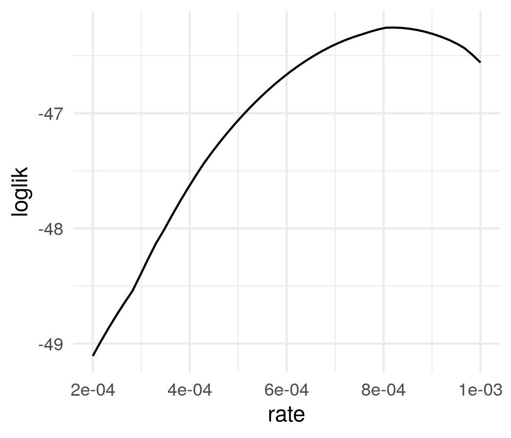
LSD is a molecular dating approach that assumes a strict clock and a fixed tree topology and branch lengths [1]. Although these are strong assumptions, LSD is extremely fast, and it has been found to perform well even when there is substantial rate variation among lineages. We estimated a phylogenetic tree for the 47 genomes using PhyML [2] and set the sampling times for calibration in LSD. We fixed the position of the root to that leading to sequence EPI_ISL_402123, shown in in Fig 1. We obtained an evolutionary rate of 2.067×10⁻⁴ subs/site/year and an age of the root node, also known as time to the most recent common ancestor (TMRCA), of early August 2019 (2019.60). Although LSD and root-to-tip regressions often produce lower rate estimates than those from Bayesian methods [3], this particular rate estimate is much lower that we would expect in coronaviruses, regardless of the method.
We also permuted the sampling times to generate a distribution of evolutionary rate estimates in the absence of an association between genetic divergence and time, known as a date-randomisation test [4,5], similar to that used by @louis.duplessis recently (Phylodynamic Analysis | 176 genomes | 6 Mar 2020 - nCoV-2019 Genomic Epidemiology - Virological). Because LSD runs in a few seconds, we can conduct a large number of randomisations in a short time, with 100 in this case. We can calculate a p-value as the proportion of randomisations with estimates that are higher than that with the correct sampling times. Following a frequentist interpretation, p<0.05 would indicate temporal signal.
The p-value here is 0.12, meaning that under this method (i.e. fixed tree topology, branch lengths and strict clocklike behaviour) there is no temporal signal, and these estimates here are probably unreliable. In particular, rate estimates for related viruses are much higher (see previous analyses in this thread), this rate is probably underestimated, leading to an overestimation of the TMRCA.
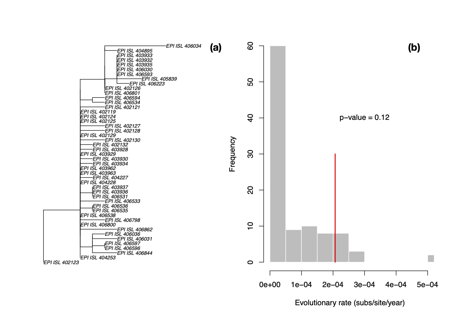
Figure 1. (a) Phylogenetic tree estimated using PhyML using HKY+Γ with root position chosen as to maximise R2 in TempEst [6]. (b) Histogram of evolutionary rate estimates along the x -axis with permuted sampling times, shown in grey, and the rate estimate with the correct sampling times, shown with the red line. The p-value indicates the proportion of randomisations with higher rate estimates than that with the correct sampling times. In a frequentist interpretation a p-value of less than 0.05 indicates temporal signal [7].
Comparing prior and posterior distributions
Another approach to assessing temporal signal that is naturally amenable to Bayesian inferences is to compare the prior and posterior distribution for parameters of interest. This is commonly done to determine the extent to which the likelihood contributes to the posterior. The rationale for this method is that a strong association between the sequence sampling times and their genetic divergence (strong temporal signal) should have a stronger influence on the posterior than when there is no temporal signal. In simulations we have found that the posterior for the age of the root should be around an order of magnitude narrower than the prior in the presence of temporal signal (BEAST 2).
We analysed the data using a strict (SC) and an uncorrelated relaxed clock with an underlying lognormal distribution (UCLN) in BEAST v1.10 [8] and a coalescent exponential tree prior. Priors for key parameters are listed in Table 1. We set a Markov chain Monte Carlo of 107 steps, sampling every 103 steps.
Table 1. Priors for key parameters used in BEAST.
| Parameter | Prior distribution |
|---|---|
| Mean rate (clockRate in the SC and ucld.mean in the UCLN) | CTMC scale prior |
| Kappa of the HKY substitution model | Lognormal, μ=1, σ=1.25 |
| Alpha of the Γ distribution | Exponential with mean=0.5 |
| Scaled population size ( Φ ; exponential.popsize) | Exponential with mean=1.0 |
| Growth rate ( r ; exponential.growthRate) | Laplace with mean=0, scale=100 |
The evolutionary rate estimates (meanRate in BEAST) from both clock models are very similar (Fig. 2), and with distributions that are substantially narrower than the prior. The mean evolutionary rate estimate for the SC model is 1.23×10⁻³ subs/site/year (95% highest posterior density, HPD: 5.63×10⁻⁴ – 1.98×10⁻³), and that for the UCLN model is 1.29×10⁻³ (HPD: 5.35×10⁻⁴ – 2.15×10⁻³).

Figure 2. Histograms of the prior and posterior evolutionary rate using the (a) SC and (b) UCLN clock models. The posterior is shown in dark blue, while the histograms with transparency and a lighter shade of blue correspond to the prior.
The age of the root is also nearly identical from both clock models and much narrower than the prior (Fig 3). The SC model estimates that the mean age of the root is mid-November 2019 (HPD: late October to mid December 2019), while the estimate from the UCLD has a mean of mid-November 2019 (HPD: late September to mid-December 2019). The 95% quantile width of the prior spans 29 years, whereas that for the posterior under either clock model is about 2 months, a strong indication of temporal signal.

Figure 3. Histograms of the prior and posterior age of the root-node (i.e. TMRCA); (a) posterior estimate from the SC, (b) posterior estimate from the UCLN, and (c) prior distribution, and (d) coefficient of rate variation of the UCLN. Note that the scale for the posterior age of root-node of the SC and UCLN are identical, whereas that for the prior is different.
A useful statistic that can be obtained from the UCLN model is the coefficient of rate variation of the evolutionary rate, which the standard deviation of branch rates divided by their mean. In general, when the posterior distribution of this statistic is abutting zero the degree of rate variation among lineages is sufficiently small as to warrant the use of a strict clock [9], although this is not a formal test of molecular clock model selection. In these data, the coefficient of rate variation is clearly abutting zero (Fig. 3). However, this does not necessarily mean that the 2019 n-Cov has clocklike behaviour, but rather that the UCLN might have an unnecessarily large number of parameters for the small data at hand.
Model tests of temporal structure (BETS)
Another Bayesian approach to assessing temporal structure consists in comparing the statistical fit of two models, one where the sequences are assigned their respective sampling times and one where the sequences are constrained to have the same sampling times. In practice, this is equivalent to comparing the fit of an isochronous and a heterochronous model. Such Bayesian Evaluation of Temporal Signal (BETS) can be performed by approximating the marginal likelihood of the two competing models and assessing their support via Bayes factors. It appears to be more powerful than the date randomisation test and the root-to-tip regression at detecting temporal signal [10]. In particular, the root-to-tip regression has been an essential tool to explore the quality of the data and to detect outliers, but it does not set a cut-off to determine the presence of temporal signal.
We conducted BETS tests using the SC and UCLN clock models and calculated the marginal likelihood using generalised stepping-stone [11,12]. An important consideration here is that all the priors should be proper (i.e. the area under the curve should be 1; Table 1). We set the marginal likelihood chain length to 105 steps, with a burn-in of 506 and with 200 path steps per β value.
Our BETS analyses strongly supported the SC model with sampling times (SC heterochronous). This model had a log Bayes factor of 5.83 over the second-best model, which was the UCLN with sampling times. Isochronous models (i.e. sequences are constrained to have the same sampling times), where the evolutionary rate is fixed to an arbitrary value had the lowest statistical fit. These results indicate that there is sufficient temporal signal in these data to allow interpretation of evolutionary rate and date estimates.
Table 2. Marginal likelihood for BETS models and estimates of evolutionary rates and time to the most recent common ancestor (TMRCA). SC stands for strict clock and ULCN for the uncorrelated relaxed clock with an underlying lognormal distribution. Heterochronous analyses are those that include sampling times, and where the evolutionary rate and TMRCA can be estimated, while in the isochronous all sequences have the same sampling times. Note that in isochronous models the evolutionary rate is fixed at an arbitrary value, and thus the rate and TMRCA are not reported.
| Model | Marginal likelihood | Evolutionary rate (subs/site/year) | TMRCA |
|---|---|---|---|
| SC heterochronous | -41028.38 | 1.23×10⁻³ (HPD: 5.63×10⁻⁴ – 1.98×10⁻³) | 2019.89 (HPD: 2019.81 – 2019.95) |
| UCLN heterochronous | -41034.21 | 1.29×10⁻³ (HPD: 5.35×10⁻⁴ – 2.15×10⁻³) | 2019.87 (HPD: 2019.74 – 2019.95) |
| UCLN isochronous | -41053.57 | - | - |
| SC isochronous | -41053.70 | - | - |
Conclusions
Our Bayesian analyses using the SC and UCLN clock models suggest that the 47 2019 n-CoV genomes available the 2nd of February of 2019 may have sufficient temporal signal. Accordingly, we infer that nCoV-2019 is evolving at a rate of around 1.26×10⁻³subs/site/year (average over the SC and UCLN model), similar to those of other human coronaviruses, and that it originated in late 2019, which is in agreement with earlier estimates by @arambaut in an earlier thread. As more data are collected, there may be stronger among-lineage rate variation as to warrant using a relaxed clock model, but we anticipate that evolutionary rates and times will be broadly similar to those estimated here.
Importantly, the molecular clock method should be carefully considered because its choice has an impact on the estimates and on the detection of temporal signal. In this situation, we found Bayesian approaches to be more powerful than LSD, probably because LSD requires more informative data (our alignment has 52 site patterns). We expect both methods to converge to similar estimates when more genomes are sequenced.
Because the outbreak recently emerged, the number of substitutions is still small, such that sequencing errors can have a considerable impact on estimates of evolutionary rates and timescales, and which can sometimes be inspected via a root-to-tip regression. Here we have taken a several precautions to mask potential sequencing errors, but these might have less of an impact when the virus accumulates more substitutions (Phylodynamic Analysis | 176 genomes | 6 Mar 2020 - nCoV-2019 Genomic Epidemiology - Virological).
References
-
To T-H, Jung M, Lycett S, Gascuel O. Fast dating using least-squares criteria and algorithms. Syst Biol. Oxford University Press; 2016;65:82–97.
-
Guindon S, Dufayard J-F, Lefort V, Anisimova M, Hordijk W, Gascuel O. New algorithms and methods to estimate maximum likelihood phylogenies: assessing the performance of PhyML 3.0. Syst Biol. 2010;59:307–21.
-
Duchêne S, Geoghegan JL, Holmes EC, Ho SYW. Estimating evolutionary rates using time-structured data: a general comparison of phylogenetic methods. Bioinformatics. 2016;32:3375–9.
-
Duchêne S, Duchêne D, Holmes EC, Ho SYW. The performance of the date-randomization test in phylogenetic analyses of time-structured virus data. Mol Biol Evol. SMBE; 2015;32:1895–906.
-
Murray GGR, Wang F, Harrison EM, Paterson GK, Mather AE, Harris SR, et al. The effect of genetic structure on molecular dating and tests for temporal signal. Methods Ecol Evol. Wiley Online Library; 2015;7:80–9.
-
Rambaut A, Lam TT, Carvalho LM, Pybus OG. Exploring the temporal structure of heterochronous sequences using TempEst (formerly Path-O-Gen). Virus Evol. The Oxford University Press; 2016;2:vew007.
-
Duchene S, Duchene DA, Geoghegan JL, Dyson ZA, Hawkey J, Holt KE. Inferring demographic parameters in bacterial genomic data using Bayesian and hybrid phylogenetic methods. BMC Evol Biol. Cold Spring Harbor Laboratory; 2018;18:95.
-
Suchard MA, Lemey P, Baele G, Ayres DL, Drummond AJ, Rambaut A. Bayesian phylogenetic and phylodynamic data integration using BEAST 1.10. Virus Evol. Oxford University Press; 2018;4:vey016.
-
Ho SS, Duchene S, Duchene DA. Simulating and detecting autocorrelation of molecular evolutionary rates among lineages. Mol Ecol Resour. 2015;15:688–96.
-
Duchene S, Stadler T, Ho SYW, Duchene DA, Dhanasekaran V, Baele G. Bayesian Evaluation of Temporal Signal in Measurably Evolving Populations. bioRxiv. Cold Spring Harbor Laboratory; 2019;810697.
-
Baele G, Lemey P, Suchard MA. Genealogical working distributions for Bayesian model testing with phylogenetic uncertainty. Syst Biol. Oxford University Press; 2016;65:250–64.
-
Fan Y, Wu R, Chen M-H, Kuo L, Lewis PO. Choosing among partition models in Bayesian phylogenetics. Mol Biol Evol. SMBE; 2011;28:523–32.
Supplementary material
Table S1. Accession numbers and GISAID labels for sequences used here. Note that EPI_ISL_406592, EPI_ISL_406595, EPI_ISL_403931, and EPI_ISL_402120 were excluded from our phylogenetic analyses.
| Sequence label | GISAID accession number |
|---|---|
| BetaCoV/Wuhan-Hu-1/2019 | EPI_ISL_402125 |
| BetaCoV/Wuhan/IPBCAMS-WH-01/2019 | EPI_ISL_402123 |
| BetaCov/Wuhan/WH01/2019 | EPI_ISL_406798 |
| BetaCoV/Wuhan/IVDC-HB-01/2019 | EPI_ISL_402119 |
| BetaCoV/Wuhan/IVDC-HB-05/2019 | EPI_ISL_402121 |
| BetaCoV/Wuhan/WIV04/2019 | EPI_ISL_402124 |
| BetaCoV/Wuhan/WIV02/2019 | EPI_ISL_402127 |
| BetaCoV/Wuhan/WIV05/2019 | EPI_ISL_402128 |
| BetaCoV/Wuhan/WIV06/2019 | EPI_ISL_402129 |
| BetaCoV/Wuhan/WIV07/2019 | EPI_ISL_402130 |
| BetaCoV/Wuhan/HBCDC-HB-01/2019 | EPI_ISL_402132 |
| BetaCoV/Wuhan/IPBCAMS-WH-04/2019 | EPI_ISL_403929 |
| BetaCoV/Wuhan/IPBCAMS-WH-03/2019 | EPI_ISL_403930 |
| BetaCoV/Wuhan/IPBCAMS-WH-02/2019 | EPI_ISL_403931 |
| BetaCoV/Shenzhen/HKU-SZ-005/2020 | EPI_ISL_405839 |
| BetaCoV/Shenzhen/HKU-SZ-002/2020 | EPI_ISL_406030 |
| BetaCoV/Wuhan/IVDC-HB-04/2020 | EPI_ISL_402120 |
| BetaCoV/Wuhan/IPBCAMS-WH-05/2020 | EPI_ISL_403928 |
| BetaCov/Wuhan/WH03/2020 | EPI_ISL_406800 |
| BetaCov/Wuhan/WH04/2020 | EPI_ISL_406801 |
| BetaCoV/Nonthaburi/61/2020 | EPI_ISL_403962 |
| BetaCoV/Nonthaburi/74/2020 | EPI_ISL_403963 |
| BetaCoV/Shenzhen/SZTH-001/2020 | EPI_ISL_406592 |
| BetaCoV/Shenzhen/SZTH-002/2020 | EPI_ISL_406593 |
| BetaCoV/Kanagawa/1/2020 | EPI_ISL_402126 |
| BetaCoV/Guangdong/20SF012/2020 | EPI_ISL_403932 |
| BetaCoV/Guangdong/20SF013/2020 | EPI_ISL_403933 |
| BetaCoV/Guangdong/20SF014/2020 | EPI_ISL_403934 |
| BetaCoV/Guangdong/20SF025/2020 | EPI_ISL_403935 |
| BetaCoV/Zhejiang/WZ-01/2020 | EPI_ISL_404227 |
| BetaCoV/Shenzhen/SZTH-003/2020 | EPI_ISL_406594 |
| BetaCoV/Shenzhen/SZTH-004/2020 | EPI_ISL_406595 |
| BetaCoV/Guangdong/20SF028/2020 | EPI_ISL_403936 |
| BetaCoV/Zhejiang/WZ-02/2020 | EPI_ISL_404228 |
| BetaCoV/Guangdong/20SF040/2020 | EPI_ISL_403937 |
| BetaCoV/USA/WA1/2020 | EPI_ISL_404895 |
| BetaCoV/USA/IL1/2020 | EPI_ISL_404253 |
| BetaCoV/USA/CA2/2020 | EPI_ISL_406036 |
| BetaCoV/USA/AZ1/2020 | EPI_ISL_406223 |
| BetaCoV/Guangdong/20SF174/2020 | EPI_ISL_406531 |
| BetaCoV/Guangzhou/20SF206/2020 | EPI_ISL_406533 |
| BetaCoV/Foshan/20SF207/2020 | EPI_ISL_406534 |
| BetaCoV/Foshan/20SF210/2020 | EPI_ISL_406535 |
| BetaCoV/Foshan/20SF211/2020 | EPI_ISL_406536 |
| BetaCoV/Taiwan/2/2020 | EPI_ISL_406031 |
| BetaCoV/USA/CA1/2020 | EPI_ISL_406034 |
| BetaCoV/Guangdong/20SF201/2020 | EPI_ISL_406538 |
| BetaCoV/France/IDF0372/2020 | EPI_ISL_406596 |
| BetaCoV/France/IDF0373/2020 | EPI_ISL_406597 |
| BetaCoV/Australia/VIC01/2020 | EPI_ISL_406844 |
| BetaCoV/Munich/BavPat1/2020 | EPI_ISL_406862 |